Configuration

PyPSA-Eur has several configuration options which are documented in this section.

Configuration Files

Any PyPSA-Eur configuration can be set in a .yaml file. The default configurations config/config.default.yaml and config/plotting.default.yaml are maintained in the repository and cover all the options that are used/ can be set.

To pass your own configuration, you can create a new file, e.g. my_config.yaml, and specify the options you want to change. They will override the default settings and options which are not set, will be inherited from the defaults above.

Another way is to use the config/config.yaml file, which does not exist in the repository and is also not tracked by git. But snakemake will always use this file if it exists. This way you can run snakemake with a custom config without having to specify the config file each time.

Configuration order of precedence is as follows: 1. Command line options specified with --config (optional) 2. Custom configuration file specified with --configfile (optional) 3. The config/config.yaml file (optional) 4. The default configuration files config/config.default.yaml and config/plotting.default.yaml

To use your custom configuration file, you need to pass it to the snakemake command using the --configfile option:

$ snakemake -call --configfile my_config.yaml

Warning

In a previous version of PyPSA-Eur (<=2025.04.0), a full copy of the created config was stored in the config/config.yaml file. This is no longer the case. If the file exists, snakemake will use it, but no new copy will be created.

Top-level configuration

“Remote” indicates the address of a server used for data exchange, often for clusters and data pushing/pulling.

version: v2025.07.0
tutorial: false

logging:
  level: INFO
  format: "%(levelname)s:%(name)s:%(message)s"

remote:
  ssh: ""
  path: ""

	Unit	Values	Description
version	–	0.x.x	Version of PyPSA-Eur. Descriptive only.
tutorial	bool	{true, false}	Switch to retrieve the tutorial data set instead of the full data set.
logging
– level	–	Any of {‘INFO’, ‘WARNING’, ‘ERROR’}	Restrict console outputs to infos, warnings, or errors only.
– format	–		Custom format for log messages. See LogRecord attributes.
remote
– ssh	–		Optionally specify the SSH of a remote cluster to be synchronized.
– path	–		Optionally specify the file path within the remote cluster to be synchronized.
secrets
– corine	–		API token for corine dataset retrieval. You can also pass the token by setting the environment variable CORINE_API_TOKEN. See scripts/retrieve_corine_dataset_primary.py for more instructions.
overpass_api
– url	–	string	Overpass API endpoint URL. See `https://wiki.openstreetmap.org/wiki/Overpass_API#Public_Overpass_API_instances`_ for available public instances.
– max_tries	–	integer	Maximum retry attempts for Overpass API requests. Please be respectful to the Overpass API fair use policy of the individual instances.
– user_agent			Please provide your own user agent details when using the Overpass API,so the instance operators can contact you if needed.
– – project_name	–	string	Project name used to identify the user agent of the Overpass API requests.
– – email	–	string	Contact email addres for the project using the Overpass API.
– – website	–	string	Website URL for the project using the Overpass API.

run

It is common conduct to analyse energy system optimisation models for multiple scenarios for a variety of reasons, e.g. assessing their sensitivity towards changing the temporal and/or geographical resolution or investigating how investment changes as more ambitious greenhouse-gas emission reduction targets are applied.

The run section is used for running and storing scenarios with different configurations which are not covered by Wildcards. It determines the path at which resources, networks and results are stored. Therefore the user can run different configurations within the same directory.

run:
  prefix: ""
  name: ""
  scenarios:
    enable: false
    file: config/scenarios.yaml
  disable_progressbar: false
  shared_resources:
    policy: false
    exclude: []
  use_shadow_directory: false

	Unit	Values	Description
name	–	str/list	Specify a name for your run. Results will be stored under this name. If scenario: enable: is set to true, the name must contain a subset of scenario names defined in scenario: file:. If the name is ‘all’, all defined scenarios will be run.
prefix	–	str	Prefix for the run name which is used as a top-layer directory name in the results and resources folders.
scenarios
– enable	bool	{true, false}	Switch to select whether workflow should generate scenarios based on file.
– file	str		Path to the scenario yaml file. The scenario file contains config overrides for each scenario. In order to be taken account, run: scenarios has to be set to true and run: name has to be a subset of top level keys given in the scenario file. In order to automatically create a scenario.yaml file based on a combination of settings, alter and use the config/create_scenarios.py script in the config directory.
disable_progressbar	bool	{true, false}	Switch to select whether progressbar should be disabled.
shared_resources
– policy	bool/str		Boolean switch to select whether resources should be shared across runs. If a string is passed, this is used as a subdirectory name for shared resources. If set to ‘base’, only resources before creating the elec.nc file are shared.
– exclude	str	For the case shared_resources=base, specify additional files that should not be shared across runs.
use_shadow_directory	bool	{true, false}	Set to true (default) if snakemake shadow directories (shallow) should be used. Set to false if problems occcur.

foresight

foresight: overnight

	Unit	Values	Description
foresight	string	{overnight, myopic, perfect}	See Foresight Options for detail explanations.

Note

If you use myopic or perfect foresight, the planning horizon in The {planning_horizons} wildcard in scenario has to be set.

scenario

The scenario section is an extraordinary section of the config file that is strongly connected to the Wildcards and is designed to facilitate running multiple scenarios through a single command

# for electricity-only studies
$ snakemake -call solve_elec_networks

# for sector-coupling studies
$ snakemake -call solve_sector_networks

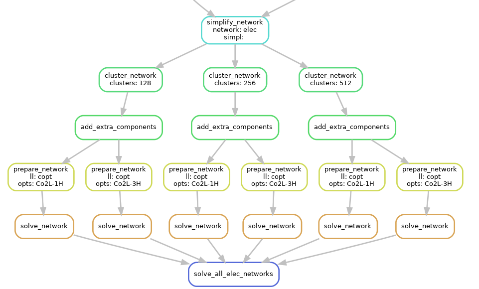
For each wildcard, a list of values is provided. The rule solve_all_elec_networks will trigger the rules for creating results/networks/base_s_{clusters}_elec_{opts}.nc for all combinations of the provided wildcard values as defined by Python’s itertools.product(…) function that snakemake’s expand(…) function uses.

An exemplary dependency graph (starting from the simplification rules) then looks like this:

scenario:
  clusters:
  - 50
  opts:
  - ''
  sector_opts:
  - ''
  planning_horizons:
  - 2050

	Unit	Values	Description
clusters	–	cf. The {clusters} wildcard	List of {clusters} wildcards to run.
opts	–	cf. The {opts} wildcard	List of {opts} wildcards to run.
sector_opts	–	cf. The {sector_opts} wildcard	List of {sector_opts} wildcards to run.
planning_horizons	–	cf. The {planning_horizons} wildcard	List of {planning_horizon} wildcards to run.

countries

countries:
- AL
- AT
- BA
- BE
- BG
- CH
- CZ
- DE
- DK
- EE
- ES
- FI
- FR
- GB
- GR
- HR
- HU
- IE
- IT
- LT
- LU
- LV
- ME
- MK
- NL
- 'NO'
- PL
- PT
- RO
- RS
- SE
- SI
- SK
- XK

	Unit	Values	Description
countries	–	Subset of {‘AL’, ‘AT’, ‘BA’, ‘BE’, ‘BG’, ‘CH’, ‘CZ’, ‘DE’, ‘DK’, ‘EE’, ‘ES’, ‘FI’, ‘FR’, ‘GB’, ‘GR’, ‘HR’, ‘HU’, ‘IE’, ‘IT’, ‘LT’, ‘LU’, ‘LV’, ‘MD’, ‘ME’, ‘MK’, ‘NL’, ‘NO’, ‘PL’, ‘PT’, ‘RO’, ‘RS’, ‘SE’, ‘SI’, ‘SK’, ‘UA’, ‘XK’}	European countries defined by their Two-letter country codes (ISO 3166-1) which should be included in the energy system model.

snapshots

Specifies the temporal range to build an energy system model for as arguments to pandas.date_range

snapshots:
  start: "2013-01-01"
  end: "2014-01-01"
  inclusive: 'left'

	Unit	Values	Description
start	–	str or list of datetime-like; e.g. YYYY-MM-DD	Left bound of date range
end	–	str or list of datetime-like; e.g. YYYY-MM-DD	Right bound of date range
inclusive	–	One of {‘neither’, ‘both’, ‘left’, ‘right’}	Make the time interval closed to the left, right, or both sides both or neither side None.

enable

Switches for some rules and optional features.

enable:
  drop_leap_day: true

	Unit	Values	Description
drop_leap_day	bool	{true, false}	Switch to drop February 29 from all time-dependent data in leap years

co2 budget

co2_budget:
  2020: 0.720 # average emissions of 2019 to 2021 relative to 1990, CO2 excl LULUCF, EEA data, European Environment Agency. (2023a). Annual European Union greenhouse gas inventory 1990–2021 and inventory report 2023 - CRF Table. https://unfccc.int/documents/627830
  2025: 0.648 # With additional measures (WAM) projection, CO2 excl LULUCF, European Environment Agency. (2023e). Member States’ greenhouse gas (GHG) emission projections 2023. https://www.eea.europa.eu/en/datahub/datahubitem-view/4b8d94a4-aed7-4e67-a54c-0623a50f48e8
  2030: 0.450 # 55% reduction by 2030 (Ff55)
  2035: 0.250
  2040: 0.100 # 90% by 2040
  2045: 0.050
  2050: 0.000 # climate-neutral by 2050

	Unit	Values	Description
co2_budget	–	Dictionary with planning horizons as keys.	CO2 budget as a fraction of 1990 emissions. Overwritten if Co2Lx or cb are set in {sector_opts} wildcard”doc/configtables/othertoplevel.csv

Note

this parameter is over-ridden if Co2Lx or cb is set in sector_opts.

electricity

electricity:
  voltages: [220., 300., 330., 380., 400., 500., 750.]
  base_network: osm
  gaslimit_enable: false
  gaslimit: false
  co2limit_enable: false
  co2limit: 7.75e+7
  co2base: 1.487e+9

  operational_reserve:
    activate: false
    epsilon_load: 0.02
    epsilon_vres: 0.02
    contingency: 4000

  max_hours:
    battery: 6
    H2: 168

  extendable_carriers:
    Generator: [solar, solar-hsat, onwind, offwind-ac, offwind-dc, offwind-float, OCGT, CCGT]
    StorageUnit: [] # battery, H2
    Store: [battery, H2]
    Link: [] # H2 pipeline

  powerplants_filter: (DateOut >= 2024 or DateOut != DateOut) and not (Country == 'Germany' and Fueltype == 'Nuclear')
  custom_powerplants: false
  everywhere_powerplants: []

  conventional_carriers: [nuclear, oil, OCGT, CCGT, coal, lignite, geothermal, biomass]
  renewable_carriers: [solar, solar-hsat, onwind, offwind-ac, offwind-dc, offwind-float, hydro]

  estimate_renewable_capacities:
    enable: true
    from_gem: true
    year: 2020
    expansion_limit: false
    technology_mapping:
      Offshore: offwind-ac
      Onshore: onwind
      PV: solar

  autarky:
    enable: false
    by_country: false

  transmission_limit: vopt

	Unit	Values	Description
voltages	kV	Any subset of {220., 300., 330., 380., 400., 500., 750.}. Distribution grid (experimental, set base_network to osm-raw): Any subset of {63., 66., 90., 110., 132., 150., 220., 300., 330., 380., 400., 500., 750.}.	Voltage levels to consider
base_network	–	Any value in {‘entsoegridkit’, ‘osm-prebuilt’, ‘osm-raw’}	Specify the underlying base network, i.e. GridKit (based on ENTSO-E web map extract, OpenStreetMap (OSM) prebuilt or raw (built from raw OSM data), takes longer.
gaslimit_enable	bool	true or false	Add an overall absolute gas limit configured in electricity: gaslimit.
gaslimit	MWhth	float or false	Global gas usage limit
co2limit_enable	bool	true or false	Add an overall absolute carbon-dioxide emissions limit configured in electricity: co2limit in prepare_network. Warning: This option should currently only be used with electricity-only networks, not for sector-coupled networks.
co2limit	\(t_{CO_2-eq}/a\)	float	Cap on total annual system carbon dioxide emissions
co2base	\(t_{CO_2-eq}/a\)	float	Reference value of total annual system carbon dioxide emissions if relative emission reduction target is specified in {opts} wildcard.
operational_reserve			Settings for reserve requirements following GenX
– activate	bool	true or false	Whether to take operational reserve requirements into account during optimisation
– epsilon_load	–	float	share of total load
– epsilon_vres	–	float	share of total renewable supply
– contingency	MW	float	fixed reserve capacity
max_hours
– battery	h	float	Maximum state of charge capacity of the battery in terms of hours at full output capacity p_nom. Cf. PyPSA documentation.
– H2	h	float	Maximum state of charge capacity of the hydrogen storage in terms of hours at full output capacity p_nom. Cf. PyPSA documentation.
extendable_carriers
– Generator	–	Any extendable carrier	Defines existing or non-existing conventional and renewable power plants to be extendable during the optimization. Conventional generators can only be built/expanded where already existent today. If a listed conventional carrier is not included in the conventional_carriers list, the lower limit of the capacity expansion is set to 0.
– StorageUnit	–	Any subset of {‘battery’,’H2’}	Adds extendable storage units (battery and/or hydrogen) at every node/bus after clustering without capacity limits and with zero initial capacity.
– Store	–	Any subset of {‘battery’,’H2’}	Adds extendable storage units (battery and/or hydrogen) at every node/bus after clustering without capacity limits and with zero initial capacity.
– Link	–	Any subset of {‘H2 pipeline’}	Adds extendable links (H2 pipelines only) at every connection where there are lines or HVDC links without capacity limits and with zero initial capacity. Hydrogen pipelines require hydrogen storage to be modelled as Store.
powerplants_filter	–	use pandas.query strings here, e.g. Country not in ['Germany']	Filter query for the default powerplant database.
custom_powerplants	–	use pandas.query strings here, e.g. Country in ['Germany']	Filter query for the custom powerplant database.
everywhere_powerplants	–	Any subset of {nuclear, oil, OCGT, CCGT, coal, lignite, geothermal, biomass}	List of conventional power plants to add to every node in the model with zero initial capacity. To be used in combination with extendable_carriers to allow for building conventional powerplants irrespective of existing locations.
conventional_carriers	–	Any subset of {nuclear, oil, OCGT, CCGT, coal, lignite, geothermal, biomass}	List of conventional power plants to include in the model from resources/powerplants_s_{clusters}.csv. If an included carrier is also listed in extendable_carriers, the capacity is taken as a lower bound.
renewable_carriers	–	Any subset of {solar, onwind, offwind-ac, offwind-dc, offwind-float, hydro}	List of renewable generators to include in the model.
estimate_renewable_capacities
– enable		bool	Activate routine to estimate renewable capacities in rule add_electricity. This option should not be used in combination with pathway planning foresight: myopic or foresight: perfect as renewable capacities are added differently in add_existing_baseyear.
– from_gem	–	bool	Add renewable capacities from Global Energy Monitor’s Global Solar Power Tracker and Global Energy Monitor’s Global Wind Power Tracker.
– year	–	bool	Renewable capacities are based on existing capacities reported by IRENA (IRENASTAT) for the specified year
– expansion_limit	–	float or false	Artificially limit maximum IRENA capacities to a factor. For example, an expansion_limit: 1.1 means 110% of capacities . If false are chosen, the estimated renewable potentials determine by the workflow are used.
– technology_mapping			Mapping between PyPSA-Eur and powerplantmatching technology names
– – Offshore	–	{onwind}	PyPSA-Eur carrier that is considered for existing onshore wind capacities (IRENA, GEM).
– – Offshore	–	Any of {offwind-ac, offwind-dc, offwind-float}	PyPSA-Eur carrier that is considered for existing offshore wind technology (IRENA, GEM).
– – PV	–	{solar}	PyPSA-Eur carrier that is considered for existing solar PV capacities (IRENA, GEM).
autarky
– enable	bool	true or false	Require each node to be autarkic by removing all lines and links.
– by_country	bool	true or false	Require each country to be autarkic by removing all cross-border lines and links. electricity: autarky must be enabled.
transmission_limit	str	Values like ‘vopt’, ‘v1.25’, ‘copt’, ‘c1.25’	Limit on transmission expansion. The first part can be v (for setting a limit on line volume) or c (for setting a limit on line cost). The second part can be opt or a float bigger than one (e.g. 1.25). If opt is chosen line expansion is optimised according to its capital cost (where the choice v only considers overhead costs for HVDC transmission lines, while c uses more accurate costs distinguishing between overhead and underwater sections and including inverter pairs). The setting v1.25 will limit the total volume of line expansion to 25% of currently installed capacities weighted by individual line lengths. The setting c1.25 will allow to build a transmission network that costs no more than 25 % more than the current system.

atlite

Define and specify the atlite.Cutout used for calculating renewable potentials and time-series. All options except for features are directly used as cutout parameters.

atlite:
  default_cutout: europe-2013-sarah3-era5
  nprocesses: 16
  show_progress: false
  cutouts:
    # use 'base' to determine geographical bounds and time span from config
    # base:
      # module: era5
    europe-2013-sarah3-era5:
      module: [sarah, era5] # in priority order
      x: [-12., 42.]
      y: [33., 72.]
      dx: 0.3
      dy: 0.3
      time: ['2013', '2013']
      # prepare_kwargs:
      #   features: []
      #   sarah_dir: ""
    europe-1940-2024-era5:
      module: era5
      x: [-12., 42.]
      y: [33., 72.]
      dx: 0.3
      dy: 0.3
      time: ['1940', '2024']
      chunks:
        time: 500
      prepare_kwargs:
        features: ['temperature', 'height', 'runoff']
        monthly_requests: true
        tmpdir: "./cutouts_tmp/"

	Unit	Values	Description
default_cutout	–	str|list	Defines a default cutout. Can refer to a single cutout or a list of cutouts.
nprocesses	–	int	Number of parallel processes in cutout preparation
show_progress	bool	true/false	Whether progressbar for atlite conversion processes should be shown. False saves time.
cutouts
– {name}	–	Convention is to name cutouts like <region>-<year>-<source> (e.g. europe-2013-sarah3-era5).	Name of the cutout netcdf file. The user may specify multiple cutouts under configuration atlite: cutouts:. Reference is used in configuration renewable: {technology}: cutout:. The cutout base may be used to automatically calculate temporal and spatial bounds of the network.
– – module	–	Subset of {‘era5’,’sarah’}	Source of the reanalysis weather dataset (e.g. ERA5 or SARAH-3)
– – x	°	Float interval within [-180, 180]	Range of longitudes to download weather data for. If not defined, it defaults to the spatial bounds of all bus shapes.
– – y	°	Float interval within [-90, 90]	Range of latitudes to download weather data for. If not defined, it defaults to the spatial bounds of all bus shapes.
– – dx	°	Larger than 0.25	Grid resolution for longitude
– – dy	°	Larger than 0.25	Grid resolution for latitude
– – time		Time interval within [‘1979’, ‘2018’] (with valid pandas date time strings)	Time span to download weather data for. If not defined, it defaults to the time interval spanned by the snapshots.
– – prepare_kwargs			Dictionary of keyword arguments passed to atlite.Cutout.prepare() when building the cutout.
– – – features		String or list of strings with valid cutout features (‘influx’, ‘wind’).	When freshly building a cutout, retrieve data only for those features. If not defined, it defaults to all available features.
– – – sarah_dir		str	Path to the location where SARAH-2 or SARAH-3 data is stored; SARAH data requires a manual separate download, see the https://atlite.readthedocs.io for details. Required for building cutouts with SARAH, not required for ERA5 cutouts.
– – – monthly_requests		bool	Whether to use monthly requests for ERA5 data when building the cutout. Helpful to avoid running into request limits with large cutouts. Defaults to False.
– – – tmpdir		str	Path to a temporary directory where intermediate files are stored when building the cutout. Helpful when building large cutouts. Defaults to None.

renewable

onwind

renewable:
  onwind:
    cutout: default
    resource:
      method: wind
      turbine: Vestas_V112_3MW
      smooth: false
      add_cutout_windspeed: true
    resource_classes: 1
    capacity_per_sqkm: 3
    # correction_factor: 0.93
    corine:
      grid_codes: [12, 13, 14, 15, 16, 17, 18, 19, 20, 21, 22, 23, 24, 25, 26, 27, 28, 29, 31, 32]
      distance: 1000
      distance_grid_codes: [1, 2, 3, 4, 5, 6]
    luisa: false
      # grid_codes: [1111, 1121, 1122, 1123, 1130, 1210, 1221, 1222, 1230, 1241, 1242]
      # distance: 1000
      # distance_grid_codes: [1111, 1121, 1122, 1123, 1130, 1210, 1221, 1222, 1230, 1241, 1242]
    natura: true
    excluder_resolution: 100
    clip_p_max_pu: 1.e-2

	Unit	Values	Description
cutout	–	str|list	Specifies the weather data cutout file(s) to use.
resource
– method	–	Must be ‘wind’	A superordinate technology type.
– turbine	–	One of turbine types included in atlite. Can be a string or a dictionary with years as keys which denote the year another turbine model becomes available.	Specifies the turbine type and its characteristic power curve.
– smooth	–	{True, False}	Switch to apply a gaussian kernel density smoothing to the power curve.
resource_classes	–	int	Number of resource classes per clustered region.
capacity_per_sqkm	\(MW/km^2\)	float	Allowable density of wind turbine placement.
corine
– grid_codes	–	Any subset of the CORINE Land Cover code list	Specifies areas according to CORINE Land Cover codes which are generally eligible for wind turbine placement.
– distance	m	float	Distance to keep from areas specified in distance_grid_codes
– distance_grid_codes	–	Any subset of the CORINE Land Cover code list	Specifies areas according to CORINE Land Cover codes to which wind turbines must maintain a distance specified in the setting distance.
luisa
– grid_codes	–	Any subset of the LUISA Base Map codes in Annex 1	Specifies areas according to the LUISA Base Map codes which are generally eligible for wind turbine placement.
– distance	m	float	Distance to keep from areas specified in distance_grid_codes
– distance_grid_codes	–	Any subset of the LUISA Base Map codes in Annex 1	Specifies areas according to the LUISA Base Map codes to which wind turbines must maintain a distance specified in the setting distance.
natura	bool	{true, false}	Switch to exclude Natura 2000 natural protection areas. Area is excluded if true.
clip_p_max_pu	p.u.	float	To avoid too small values in the renewables` per-unit availability time series values below this threshold are set to zero.
correction_factor	–	float	Correction factor for capacity factor time series.
excluder_resolution	m	float	Resolution on which to perform geographical elibility analysis.

Note

Notes on capacity_per_sqkm. ScholzPhd Tab 4.3.1: 10MW/km^2 and assuming 30% fraction of the already restricted area is available for installation of wind generators due to competing land use and likely public acceptance issues.

Note

The default choice for corine grid_codes was based on Scholz, Y. (2012). Renewable energy based electricity supply at low costs development of the REMix model and application for Europe. ( p.42 / p.28)

offwind-x

  offwind-ac:
    cutout: default
    resource:
      method: wind
      turbine: NREL_ReferenceTurbine_2020ATB_5.5MW
      smooth: false
      add_cutout_windspeed: true
    resource_classes: 1
    capacity_per_sqkm: 2
    correction_factor: 0.8855
    corine: [44, 255]
    luisa: false # [0, 5230]
    natura: true
    ship_threshold: 400
    max_depth: 60
    max_shore_distance: 30000
    excluder_resolution: 200
    clip_p_max_pu: 1.e-2
    landfall_length: 20
  offwind-dc:
    cutout: default
    resource:
      method: wind
      turbine: NREL_ReferenceTurbine_2020ATB_5.5MW
      smooth: false
      add_cutout_windspeed: true
    resource_classes: 1
    capacity_per_sqkm: 2
    correction_factor: 0.8855
    corine: [44, 255]
    luisa: false # [0, 5230]
    natura: true
    ship_threshold: 400
    max_depth: 60
    min_shore_distance: 30000
    excluder_resolution: 200
    clip_p_max_pu: 1.e-2
    landfall_length: 30
  offwind-float:
    cutout: default
    resource:
      method: wind
      turbine: NREL_ReferenceTurbine_5MW_offshore
      smooth: false
      add_cutout_windspeed: true
    resource_classes: 1
    # ScholzPhd Tab 4.3.1: 10MW/km^2
    capacity_per_sqkm: 2
    correction_factor: 0.8855
    # proxy for wake losses
    # from 10.1016/j.energy.2018.08.153
    # until done more rigorously in #153
    corine: [44, 255]
    natura: true
    ship_threshold: 400
    excluder_resolution: 200
    min_depth: 60
    max_depth: 1000
    clip_p_max_pu: 1.e-2
    landfall_length: 40

	Unit	Values	Description
cutout	–	str|list	Specifies the weather data cutout file(s) to use.
resource
– method	–	Must be ‘wind’	A superordinate technology type.
– turbine	–	One of turbine types included in atlite. Can be a string or a dictionary with years as keys which denote the year another turbine model becomes available.	Specifies the turbine type and its characteristic power curve.
– smooth	–	{True, False}	Switch to apply a gaussian kernel density smoothing to the power curve.
resource_classes	–	int	Number of resource classes per clustered region.
capacity_per_sqkm	\(MW/km^2\)	float	Allowable density of wind turbine placement.
correction_factor	–	float	Correction factor for capacity factor time series.
excluder_resolution	m	float	Resolution on which to perform geographical elibility analysis.
corine	–	Any realistic subset of the CORINE Land Cover code list	Specifies areas according to CORINE Land Cover codes which are generally eligible for AC-connected offshore wind turbine placement.
luisa	–	Any subset of the LUISA Base Map codes in Annex 1	Specifies areas according to the LUISA Base Map codes which are generally eligible for AC-connected offshore wind turbine placement.
natura	bool	{true, false}	Switch to exclude Natura 2000 natural protection areas. Area is excluded if true.
ship_threshold	–	float	Ship density threshold from which areas are excluded.
max_depth	m	float	Maximum sea water depth at which wind turbines can be build. Maritime areas with deeper waters are excluded in the process of calculating the AC-connected offshore wind potential.
min_shore_distance	m	float	Minimum distance to the shore below which wind turbines cannot be build. Such areas close to the shore are excluded in the process of calculating the AC-connected offshore wind potential.
max_shore_distance	m	float	Maximum distance to the shore above which wind turbines cannot be build. Such areas close to the shore are excluded in the process of calculating the AC-connected offshore wind potential.
clip_p_max_pu	p.u.	float	To avoid too small values in the renewables` per-unit availability time series values below this threshold are set to zero.
landfall_length	km	float	Fixed length of the cable connection that is onshorelandfall in km. If ‘centroid’, the length is calculated as the distance to centroid of the onshore bus.

Note

Notes on capacity_per_sqkm. ScholzPhd Tab 4.3.1: 10MW/km^2 and assuming 20% fraction of the already restricted area is available for installation of wind generators due to competing land use and likely public acceptance issues.

Note

Notes on correction_factor. Correction due to proxy for wake losses from 10.1016/j.energy.2018.08.153 until done more rigorously in #153

solar

  solar:
    cutout: default
    resource:
      method: pv
      panel: CSi
      orientation:
        slope: 35.
        azimuth: 180.
    resource_classes: 1
    capacity_per_sqkm: 5.1
    # correction_factor: 0.854337
    corine: [1, 2, 3, 4, 5, 6, 7, 8, 9, 10, 11, 12, 13, 14, 15, 16, 17, 18, 19, 20, 26, 31, 32]
    luisa: false # [1111, 1121, 1122, 1123, 1130, 1210, 1221, 1222, 1230, 1241, 1242, 1310, 1320, 1330, 1410, 1421, 1422, 2110, 2120, 2130, 2210, 2220, 2230, 2310, 2410, 2420, 3210, 3320, 3330]
    natura: true
    excluder_resolution: 100
    clip_p_max_pu: 1.e-2
  solar-hsat:
    cutout: default
    resource:
      method: pv
      panel: CSi
      orientation:
        slope: 35.
        azimuth: 180.
      tracking: horizontal
    resource_classes: 1
    capacity_per_sqkm: 4.43 # 15% higher land usage acc. to NREL
    corine: [1, 2, 3, 4, 5, 6, 7, 8, 9, 10, 11, 12, 13, 14, 15, 16, 17, 18, 19, 20, 26, 31, 32]
    luisa: false # [1111, 1121, 1122, 1123, 1130, 1210, 1221, 1222, 1230, 1241, 1242, 1310, 1320, 1330, 1410, 1421, 1422, 2110, 2120, 2130, 2210, 2220, 2230, 2310, 2410, 2420, 3210, 3320, 3330]
    natura: true
    excluder_resolution: 100
    clip_p_max_pu: 1.e-2

	Unit	Values	Description
cutout	–	str|list	Specifies the weather data cutout file(s) to use.
resource
– method	–	Must be ‘pv’	A superordinate technology type.
– panel	–	One of {‘Csi’, ‘CdTe’, ‘KANENA’} as defined in atlite . Can be a string or a dictionary with years as keys which denote the year another turbine model becomes available.	Specifies the solar panel technology and its characteristic attributes.
– orientation
– – slope	°	Realistically any angle in [0., 90.]	Specifies the tilt angle (or slope) of the solar panel. A slope of zero corresponds to the face of the panel aiming directly overhead. A positive tilt angle steers the panel towards the equator.
– – azimuth	°	Any angle in [0., 360.]	Specifies the azimuth orientation of the solar panel. South corresponds to 180.°.
resource_classes	–	int	Number of resource classes per clustered region.
capacity_per_sqkm	\(MW/km^2\)	float	Allowable density of solar panel placement.
correction_factor	–	float	A correction factor for the capacity factor (availability) time series.
corine	–	Any subset of the CORINE Land Cover code list	Specifies areas according to CORINE Land Cover codes which are generally eligible for solar panel placement.
luisa	–	Any subset of the LUISA Base Map codes in Annex 1	Specifies areas according to the LUISA Base Map codes which are generally eligible for solar panel placement.
natura	bool	{true, false}	Switch to exclude Natura 2000 natural protection areas. Area is excluded if true.
clip_p_max_pu	p.u.	float	To avoid too small values in the renewables` per-unit availability time series values below this threshold are set to zero.
excluder_resolution	m	float	Resolution on which to perform geographical elibility analysis.

Note

Notes on capacity_per_sqkm. ScholzPhd Tab 4.3.1: 170 MW/km^2 and assuming 1% of the area can be used for solar PV panels. Correction factor determined by comparing uncorrected area-weighted full-load hours to those published in Supplementary Data to Pietzcker, Robert Carl, et al. “Using the sun to decarbonize the power sector – The economic potential of photovoltaics and concentrating solar power.” Applied Energy 135 (2014): 704-720. This correction factor of 0.854337 may be in order if using reanalysis data. for discussion refer to this <issue PyPSA/pypsa-eur#285>

hydro

  hydro:
    cutout: default
    carriers: [ror, PHS, hydro]
    PHS_max_hours: 6
    hydro_max_hours: energy_capacity_totals_by_country # one of energy_capacity_totals_by_country, estimate_by_large_installations or a float
    flatten_dispatch: false
    flatten_dispatch_buffer: 0.2
    clip_min_inflow: 1.0
    eia_norm_year: false
    eia_correct_by_capacity: false
    eia_approximate_missing: false

	Unit	Values	Description
cutout	–	str|list	Specifies the weather data cutout file(s) to use.
carriers	–	Any subset of {‘ror’, ‘PHS’, ‘hydro’}	Specifies the types of hydro power plants to build per-unit availability time series for. ‘ror’ stands for run-of-river plants, ‘PHS’ represents pumped-hydro storage, and ‘hydro’ stands for hydroelectric dams.
PHS_max_hours	h	float	Maximum state of charge capacity of the pumped-hydro storage (PHS) in terms of hours at full output capacity p_nom. Cf. PyPSA documentation.
hydro_max_hours	h	Any of {float, ‘energy_capacity_totals_by_country’, ‘estimate_by_large_installations’}	Maximum state of charge capacity of the pumped-hydro storage (PHS) in terms of hours at full output capacity p_nom or heuristically determined. Cf. PyPSA documentation.
flatten_dispatch	bool	{true, false}	Consider an upper limit for the hydro dispatch. The limit is given by the average capacity factor plus the buffer given in flatten_dispatch_buffer
flatten_dispatch_buffer	–	float	If flatten_dispatch is true, specify the value added above the average capacity factor.
clip_min_inflow	MW	float	To avoid too small values in the inflow time series, values below this threshold are set to zero.
eia_norm_year	–	Year in EIA hydro generation dataset; or False to disable	To specify a specific year by which hydro inflow is normed that deviates from the snapshots’ year
eia_correct_by_capacity	–	boolean	Correct EIA annual hydro generation data by installed capacity.
eia_approximate_missing	–	boolean	Approximate hydro generation data for years not included in EIA dataset through a regression based on annual runoff.

conventional

Define additional generator attribute for conventional carrier types. If a scalar value is given it is applied to all generators. However if a string starting with “data/” is given, the value is interpreted as a path to a csv file with country specific values. Then, the values are read in and applied to all generators of the given carrier in the given country. Note that the value(s) overwrite the existing values.

conventional:
  unit_commitment: false
  dynamic_fuel_price: false
  nuclear:
    p_max_pu: data/nuclear_p_max_pu.csv # float of file name

	Unit	Values	Description
unit_commitment	bool	{true, false}	Allow the overwrite of ramp_limit_up, ramp_limit_start_up, ramp_limit_shut_down, p_min_pu, min_up_time, min_down_time, and start_up_cost of conventional generators. Refer to the CSV file „unit_commitment.csv“.
dynamic_fuel_price	bool	{true, false}	Consider the monthly fluctuating fuel prices for each conventional generator. Refer to the CSV file “data/validation/monthly_fuel_price.csv”.
{name}	–	string	For any carrier/technology overwrite attributes as listed below.
– {attribute}	–	string or float	For any attribute, can specify a float or reference to a file path to a CSV file giving floats for each country (2-letter code).

lines

lines:
  types:
    63.: 94-AL1/15-ST1A 20.0
    66.: 94-AL1/15-ST1A 20.0
    90.: 184-AL1/30-ST1A 110.0
    110.: 184-AL1/30-ST1A 110.0
    132.: 243-AL1/39-ST1A 110.0
    150.: 243-AL1/39-ST1A 110.0
    220.: Al/St 240/40 2-bundle 220.0
    300.: Al/St 240/40 3-bundle 300.0
    330.: Al/St 240/40 3-bundle 300.0
    380.: Al/St 240/40 4-bundle 380.0
    400.: Al/St 240/40 4-bundle 380.0
    500.: Al/St 240/40 4-bundle 380.0
    750.: Al/St 560/50 4-bundle 750.0
  s_max_pu: 0.7
  s_nom_max: .inf
  max_extension: 20000 #MW
  length_factor: 1.25
  reconnect_crimea: true
  under_construction: keep # 'zero': set capacity to zero, 'remove': remove, 'keep': with full capacity for lines in grid extract
  dynamic_line_rating:
    activate: false
    cutout: default
    correction_factor: 0.95
    max_voltage_difference: false
    max_line_rating: false

	Unit	Values	Description
types	–	Values should specify a line type in PyPSA. Keys should specify the corresponding voltage level (e.g. 220., 300. and 380. kV)	Specifies line types to assume for the different voltage levels of the ENTSO-E grid extraction. Should normally handle voltage levels 220, 300, and 380 kV
s_max_pu	–	Value in [0.,1.]	Correction factor for line capacities (s_nom) to approximate \(N-1\) security and reserve capacity for reactive power flows
s_nom_max	MW	float	Global upper limit for the maximum capacity of each extendable line.
max_extension	MW	float	Upper limit for the extended capacity of each extendable line.
length_factor	–	float	Correction factor to account for the fact that buses are not connected by lines through air-line distance.
under_construction	–	One of {‘zero’: set capacity to zero, ‘remove’: remove completely, ‘keep’: keep with full capacity}	Specifies how to handle lines which are currently under construction.
reconnect_crimea	–	true or false	Whether to reconnect Crimea to the Ukrainian grid
dynamic_line_rating
– activate	bool	true or false	Whether to take dynamic line rating into account
– cutout	–	str|list	Specifies the weather data cutout file(s) to use.
– correction_factor	–	float	Factor to compensate for overestimation of wind speeds in hourly averaged wind data
– max_voltage_difference	deg	float	Maximum voltage angle difference in degrees or ‘false’ to disable
– max_line_rating	–	float	Maximum line rating relative to nominal capacity without DLR, e.g. 1.3 or ‘false’ to disable

links

links:
  p_max_pu: 1.0
  p_min_pu: -1.0
  p_nom_max: .inf
  max_extension: 30000 #MW
  length_factor: 1.25
  under_construction: keep # 'zero': set capacity to zero, 'remove': remove, 'keep': with full capacity for lines in grid extract

	Unit	Values	Description
p_max_pu	–	Value in [0.,1.]	Correction factor for link capacities p_nom.
p_min_pu	–	Value in [-1.,0.]	Correction factor for link capacities p_nom.
p_nom_max	MW	float	Global upper limit for the maximum capacity of each extendable DC link.
max_extension	MW	float	Upper limit for the extended capacity of each extendable DC link.
length_factor	–	float	Correction factor to account for the fact that buses are not connected by links through air-line distance.
under_construction	–	One of {‘zero’: set capacity to zero, ‘remove’: remove completely, ‘keep’: keep with full capacity}	Specifies how to handle lines which are currently under construction.

transmission projects

Allows to define additional transmission projects that will be added to the base network, e.g., from the TYNDP 2020 dataset. The projects are read in from the CSV files in the subfolder of data/transmission_projects/. New transmission projects, e.g. from TYNDP 2024, can be added in a new subfolder of transmission projects, e.g. data/transmission_projects/tyndp2024 while extending the list of transmission_projects in the config.yaml by tyndp2024. The CSV files in the project folder should have the same columns as the CSV files in the template folder data/transmission_projects/template.

transmission_projects:
  enable: true
  include:
    tyndp2020: true
    nep: true
    manual: true
  skip:
  - upgraded_lines
  - upgraded_links
  status:
  - under_construction
  - in_permitting
  - confirmed
    #- planned_not_yet_permitted
    #- under_consideration
  new_link_capacity: zero #keep or zero

	Unit	Values	Description
enable	bool	{true,false}	Whether to integrate this transmission projects or not.
include	–		Name of the transmission projects. They should be unique and have to be provided in the data/transmission_projects folder.
– tyndp2020	bool	{true,false}	Whether to integrate the TYNDP 2020 dataset.
– nep	bool	{true,false}	Whether to integrate the German network development plan dataset.
– manual	bool	{true,false}	Whether to integrate the manually added transmission projects. They are taken from the previously existing links_tyndp.csv file.
skip	list		Type of lines to skip from all transmission projects. Possible values are: upgraded_lines, upgraded_links, new_lines, new_links.
status	list or dict		Status to include into the model as list or as dict with name of project and status to include. Possible values for status are under_construction, in_permitting, confirmed, planned_not_yet_permitted, under_consideration.
new_link_capacity	–	{zero,keep}	Whether to set the new link capacity to the provided capacity or set it to zero.

transformers

transformers:
  x: 0.1
  s_nom: 2000.
  type: ''

	Unit	Values	Description
x	p.u.	float	Series reactance (per unit, using s_nom as base power of the transformer. Overwritten if type is specified.
s_nom	MVA	float	Limit of apparent power which can pass through branch. Overwritten if type is specified.
type	–	A transformer type in PyPSA.	Specifies transformer types to assume for the transformers of the ENTSO-E grid extraction.

load

load:
  fill_gaps:
    enable: true
    interpolate_limit: 3
    time_shift_for_large_gaps: 1w
  manual_adjustments: true
  scaling_factor: 1.0
  fixed_year: false
  supplement_synthetic: true
  distribution_key:
    gdp: 0.6
    population: 0.4

	Unit	Values	Description
fill_gaps	–	–	Gaps filling strategy used.
– enable	bool	{true, false}	Whether to fill gaps using interpolation for small gaps and time shift for large gaps.
– interpolate_limit	hours	integer	Maximum gap size (consecutive nans) which interpolated linearly.
– time_shift_for_large_gaps	string	string	Periods which are used for copying time-slices in order to fill large gaps of nans. Have to be valid pandas period strings.
manual_adjustments	bool	{true, false}	Whether to adjust the load data manually according to the function in manual_adjustment().
scaling_factor	–	float	Global correction factor for the load time series.
fixed_year	–	Year or False	To specify a fixed year for the load time series that deviates from the snapshots’ year
supplement_synthetic	bool	{true, false}	Whether to supplement missing data for selected time period should be supplemented by synthetic data from https://zenodo.org/records/10820928.
distribution_key	–	–	Distribution key for spatially disaggregating the per-country electricity demand data.
– gdp	float	[0, 1]	Weighting factor for the GDP data in the distribution key.
– population	float	[0, 1]	Weighting factor for the population data in the distribution key.

energy

Note

Only used for sector-coupling studies.

energy:
  energy_totals_year: 2019
  base_emissions_year: 1990
  emissions: CO2

	Unit	Values	Description
energy_totals_year	–	{1990,1995,2000,2005,2010,2011,…}	The year for the sector energy use. The year must be avaliable in the Eurostat report
base_emissions_year	–	YYYY; e.g. 1990	The base year for the sector emissions. See European Environment Agency (EEA).
emissions	–	{CO2, All greenhouse gases - (CO2 equivalent)}	Specify which sectoral emissions are taken into account. Data derived from EEA. Currently only CO2 is implemented.

biomass

Note

Only used for sector-coupling studies.

biomass:
  year: 2030
  scenario: ENS_Med
  classes:
    solid biomass:
    - Agricultural waste
    - Fuelwood residues
    - Secondary Forestry residues - woodchips
    - Sawdust
    - Residues from landscape care
    not included:
    - Sugar from sugar beet
    - Rape seed
    - "Sunflower, soya seed "
    - Bioethanol barley, wheat, grain maize, oats, other cereals and rye
    - Miscanthus, switchgrass, RCG
    - Willow
    - Poplar
    - FuelwoodRW
    - C&P_RW
    biogas:
    - Manure solid, liquid
    - Sludge
    municipal solid waste:
    - Municipal waste
  share_unsustainable_use_retained:
    2020: 1
    2025: 1
    2030: 0.66
    2035: 0.33
    2040: 0
    2045: 0
    2050: 0
  share_sustainable_potential_available:
    2020: 0
    2025: 0
    2030: 0.33
    2035: 0.66
    2040: 1
    2045: 1
    2050: 1

	Unit	Values	Description
year	–	{2010, 2020, 2030, 2040, 2050}	Year for which to retrieve biomass potential according to the assumptions of the JRC ENSPRESO .
scenario	–	{“ENS_Low”, “ENS_Med”, “ENS_High”}	Scenario for which to retrieve biomass potential. The scenario definition can be seen in ENSPRESO_BIOMASS
classes
– solid biomass	–	Array of biomass comodity	The comodity that are included as solid biomass
– not included	–	Array of biomass comodity	The comodity that are not included as a biomass potential
– biogas	–	Array of biomass comodity	The comodity that are included as biogas
share_unsustainable_use_retained	–	Dictionary with planning horizons as keys.	Share of unsustainable biomass use retained using primary production of Eurostat data as reference
share_sustainable_potential_available	–	Dictionary with planning horizons as keys.	Share determines phase-in of ENSPRESO biomass potentials

The list of available biomass is given by the category in ENSPRESO_BIOMASS, namely:

• Agricultural waste

• Manure solid, liquid

• Residues from landscape care

• Bioethanol barley, wheat, grain maize, oats, other cereals and rye

• Sugar from sugar beet

• Miscanthus, switchgrass, RCG

• Willow

• Poplar

• Sunflower, soya seed

• Rape seed

• Fuelwood residues

• FuelwoodRW

• C&P_RW

• Secondary Forestry residues - woodchips

• Sawdust

• Municipal waste

• Sludge

solar_thermal

Note

Only used for sector-coupling studies.

solar_thermal:
  clearsky_model: simple  # should be "simple" or "enhanced"?
  orientation:
    slope: 45.
    azimuth: 180.
  cutout: default

	Unit	Values	Description
clearsky_model	–	{‘simple’, ‘enhanced’}	Type of clearsky model for diffuse irradiation
orientation	–	{units of degrees, ‘latitude_optimal’}	Panel orientation with slope and azimuth
– azimuth	float	units of degrees	The angle between the North and the sun with panels on the local horizon
– slope	float	units of degrees	The angle between the ground and the panels

existing_capacities

Note

Only used for sector-coupling studies. The value for grouping years are only used in myopic or perfect foresight scenarios.

existing_capacities:
  grouping_years_power: [1920, 1950, 1955, 1960, 1965, 1970, 1975, 1980, 1985, 1990, 1995, 2000, 2005, 2010, 2015, 2020, 2025]
  grouping_years_heat: [1980, 1985, 1990, 1995, 2000, 2005, 2010, 2015, 2019] # heat grouping years >= baseyear will be ignored
  threshold_capacity: 10
  default_heating_lifetime: 20
  conventional_carriers:
  - lignite
  - coal
  - oil
  - uranium

	Unit	Values	Description
grouping_years_power	–	A list of years	Intervals to group existing capacities for power
grouping_years_heat	–	A list of years below 2020	Intervals to group existing capacities for heat
threshold_capacity	MW	float	Capacities generators and links of below threshold are removed during add_existing_capacities
default_heating_lifetime	years	int	Default lifetime for heating technologies
conventional_carriers	–	Any subset of {uranium, coal, lignite, oil}	List of conventional power plants to include in the sectoral network

sector

Note

Only used for sector-coupling studies.

sector:
  transport: true
  heating: true
  biomass: true
  industry: true
  shipping: true
  aviation: true
  agriculture: true
  fossil_fuels: true
  district_heating:
    potential: 0.6
    progress:
      2020: 0.0
      2025: 0.1
      2030: 0.25
      2035: 0.4
      2040: 0.55
      2045: 0.75
      2050: 1.0
    district_heating_loss: 0.15
    supply_temperature_approximation:
      max_forward_temperature_baseyear:
        FR: 110
        DK: 75
        DE: 109
        CZ: 130
        FI: 115
        PL: 130
        SE: 102
        IT: 90
      min_forward_temperature_baseyear:
        DE: 82
      return_temperature_baseyear:
        DE: 58
      lower_threshold_ambient_temperature: 0
      upper_threshold_ambient_temperature: 10
      rolling_window_ambient_temperature: 72
      relative_annual_temperature_reduction: 0.01
    ptes:
      dynamic_capacity: false
      supplemental_heating:
        enable: false
        booster_heat_pump: false
      max_top_temperature: 90
      min_bottom_temperature: 35
    ates:
      enable: false
      suitable_aquifer_types:
      - Highly productive porous aquifers
      aquifer_volumetric_heat_capacity: 2600
      fraction_of_aquifer_area_available: 0.2
      effective_screen_length: 20
      capex_as_fraction_of_geothermal_heat_source: 0.75
      recovery_factor: 0.6
      marginal_cost_charger: 0.035
      ignore_missing_regions: false
    heat_source_cooling: 6 #K
    heat_pump_cop_approximation:
      refrigerant: ammonia
      heat_exchanger_pinch_point_temperature_difference: 5 #K
      isentropic_compressor_efficiency: 0.8
      heat_loss: 0.0
      min_delta_t_lift: 10 #K
    limited_heat_sources:
      geothermal:
        constant_temperature_celsius: 65
        ignore_missing_regions: false
      river_water:
        constant_temperature_celsius: false
    direct_utilisation_heat_sources:
    - geothermal
    temperature_limited_stores:
    - ptes
    dh_areas:
      buffer: 1000
      handle_missing_countries: fill
  heat_pump_sources:
    urban central:
    - air
    urban decentral:
    - air
    rural:
    - air
    - ground
  residential_heat:
    dsm:
      enable: false
      direction:
      - overheat
      - undercool
      restriction_value:
        2020: 0.06
        2025: 0.16
        2030: 0.27
        2035: 0.36
        2040: 0.38
        2045: 0.39
        2050: 0.4
      restriction_time:
      - 10
      - 22
  cluster_heat_buses: true
  heat_demand_cutout: default
  bev_dsm_restriction_value: 0.8
  bev_dsm_restriction_time: 7
  transport_heating_deadband_upper: 20.
  transport_heating_deadband_lower: 15.
  ICE_lower_degree_factor: 0.375
  ICE_upper_degree_factor: 1.6
  EV_lower_degree_factor: 0.98
  EV_upper_degree_factor: 0.63
  bev_dsm: true
  bev_dsm_availability: 0.5
  bev_energy: 0.05
  bev_charge_efficiency: 0.9
  bev_charge_rate: 0.011
  bev_avail_max: 0.95
  bev_avail_mean: 0.8
  v2g: true
  land_transport_fuel_cell_share:
    2020: 0
    2025: 0
    2030: 0
    2035: 0
    2040: 0
    2045: 0
    2050: 0
  land_transport_electric_share:
    2020: 0
    2025: 0.05
    2030: 0.2
    2035: 0.45
    2040: 0.7
    2045: 0.85
    2050: 1
  land_transport_ice_share:
    2020: 1
    2025: 0.95
    2030: 0.8
    2035: 0.55
    2040: 0.3
    2045: 0.15
    2050: 0
  transport_electric_efficiency: 53.19 # 1 MWh_el = 53.19*100 km
  transport_fuel_cell_efficiency: 30.003 # 1 MWh_H2 = 30.003*100 km
  transport_ice_efficiency: 16.0712 # 1 MWh_oil = 16.0712 * 100 km
  agriculture_machinery_electric_share: 0.5
  agriculture_machinery_oil_share: 0.5
  agriculture_machinery_fuel_efficiency: 0.7
  agriculture_machinery_electric_efficiency: 0.3
  MWh_MeOH_per_MWh_H2: 0.8787
  MWh_MeOH_per_tCO2: 4.0321
  MWh_MeOH_per_MWh_e: 3.6907
  shipping_hydrogen_liquefaction: false
  shipping_hydrogen_share:
    2020: 0
    2025: 0
    2030: 0
    2035: 0
    2040: 0
    2045: 0
    2050: 0
  shipping_methanol_share:
    2020: 0
    2025: 0
    2030: 0.15
    2035: 0.35
    2040: 0.55
    2045: 0.8
    2050: 1
  shipping_oil_share:
    2020: 1
    2025: 1
    2030: 0.85
    2035: 0.65
    2040: 0.45
    2045: 0.2
    2050: 0
  shipping_methanol_efficiency: 0.46
  shipping_oil_efficiency: 0.40
  aviation_demand_factor: 1.
  HVC_demand_factor: 1.
  time_dep_hp_cop: true
  heat_pump_sink_T_individual_heating: 55.
  reduce_space_heat_exogenously: true
  reduce_space_heat_exogenously_factor:
    2020: 0.10  # this results in a space heat demand reduction of 10%
    2025: 0.09  # first heat demand increases compared to 2020 because of larger floor area per capita
    2030: 0.09
    2035: 0.11
    2040: 0.16
    2045: 0.21
    2050: 0.29
  retrofitting:
    retro_endogen: false
    cost_factor: 1.0
    interest_rate: 0.04
    annualise_cost: true
    tax_weighting: false
    construction_index: true
  tes: true
  boilers: true
  resistive_heaters: true
  oil_boilers: false
  biomass_boiler: true
  overdimension_heat_generators:
    decentral: 1.1  #to cover demand peaks bigger than data
    central: 1.0
  chp:
    enable: true
    fuel:
    - solid biomass # For solid biomass, CHP with and without CC are added
    - gas # For all other fuels the same techno economic data from gas CHP is taken
    micro_chp: false # Only gas is used for micro_chp
  solar_thermal: true
  solar_cf_correction: 0.788457  # =  >>> 1/1.2683
  methanation: true
  coal_cc: false
  dac: true
  co2_vent: false
  heat_vent:
    urban central: true
    urban decentral: true
    rural: true
  marginal_cost_heat_vent: 0.02
  allam_cycle_gas: false
  hydrogen_fuel_cell: true
  hydrogen_turbine: true
  SMR: true
  SMR_cc: true
  regional_oil_demand: true
  regional_coal_demand: false
  regional_co2_sequestration_potential:
    enable: true
    attribute:
    - conservative estimate Mt
    - conservative estimate GAS Mt
    - conservative estimate OIL Mt
    - conservative estimate aquifer Mt
    include_onshore: false
    min_size: 3
    max_size: 25
    years_of_storage: 25
  co2_sequestration_potential:
    2020: 0
    2025: 0
    2030: 40
    2035: 100
    2040: 180
    2045: 250
    2050: 250
  co2_sequestration_cost: 30
  co2_sequestration_lifetime: 50
  co2_spatial: true
  co2_network: true
  co2_network_cost_factor: 1
  cc_fraction: 0.9
  hydrogen_underground_storage: true
  hydrogen_underground_storage_locations:
  - onshore    # more than 50 km from sea
  - nearshore      # within 50 km of sea
    # - offshore
  methanol:
    regional_methanol_demand: false
    methanol_reforming: false
    methanol_reforming_cc: false
    methanol_to_kerosene: false
    methanol_to_power:
      ccgt: false
      ccgt_cc: false
      ocgt: true
      allam: false
    biomass_to_methanol: true
    biomass_to_methanol_cc: false
  ammonia: true
  min_part_load_electrolysis: 0
  min_part_load_fischer_tropsch: 0.5
  min_part_load_methanolisation: 0.3
  min_part_load_methanation: 0.3
  use_fischer_tropsch_waste_heat: 0.25
  use_haber_bosch_waste_heat: 0.25
  use_methanolisation_waste_heat: 0.25
  use_methanation_waste_heat: 0.25
  use_fuel_cell_waste_heat: 1
  use_electrolysis_waste_heat: 0.25
  electricity_transmission_grid: true
  electricity_distribution_grid: true
  electricity_grid_connection: true
  transmission_efficiency:
    enable:
    - DC
    - H2 pipeline
    - gas pipeline
    - electricity distribution grid
    DC:
      efficiency_static: 0.98
      efficiency_per_1000km: 0.977
    H2 pipeline:
      efficiency_per_1000km: 1 # 0.982
      compression_per_1000km: 0.018
    gas pipeline:
      efficiency_per_1000km: 1 #0.977
      compression_per_1000km: 0.01
    electricity distribution grid:
      efficiency_static: 0.97
  H2_network: true
  gas_network: true
  H2_retrofit: false
  H2_retrofit_capacity_per_CH4: 0.6
  gas_network_connectivity_upgrade: 1
  gas_distribution_grid: true
  gas_distribution_grid_cost_factor: 1.0
  biomass_spatial: true
  biomass_transport: false
  biogas_upgrading: true
  biogas_upgrading_cc: false
  conventional_generation:
    OCGT: gas
    CCGT: gas
  biomass_to_liquid: true
  biomass_to_liquid_cc: false
  electrobiofuels: true
  biosng: false
  biosng_cc: false
  bioH2: false
  municipal_solid_waste: false
  limit_max_growth:
    enable: false
    # allowing 30% larger than max historic growth
    factor: 1.3
    max_growth:  # unit GW
      onwind: 16 # onshore max grow so far 16 GW in Europe https://www.iea.org/reports/renewables-2020/wind
      solar: 28 # solar max grow so far 28 GW in Europe https://www.iea.org/reports/renewables-2020/solar-pv
      offwind-ac: 35 # offshore max grow so far 3.5 GW in Europe https://windeurope.org/about-wind/statistics/offshore/european-offshore-wind-industry-key-trends-statistics-2019/
      offwind-dc: 35
    max_relative_growth:
      onwind: 3
      solar: 3
      offwind-ac: 3
      offwind-dc: 3
  enhanced_geothermal:
    enable: false
    flexible: true
    max_hours: 240
    max_boost: 0.25
    var_cf: true
    sustainability_factor: 0.0025
  solid_biomass_import:
    enable: false
    price: 54 #EUR/MWh
    max_amount: 1390 # TWh
    upstream_emissions_factor: .1 #share of solid biomass CO2 emissions at full combustion
  imports:
    enable: false
    limit: .inf
    limit_sense: <=
    price:
      H2: 74
      NH3: 97
      methanol: 121
      gas: 122
      oil: 125

industry

Note

Only used for sector-coupling studies.

# docs in https://pypsa-eur.readthedocs.io/en/latest/configuration.html#industry
industry:
  St_primary_fraction:
    2020: 0.6
    2025: 0.55
    2030: 0.5
    2035: 0.45
    2040: 0.4
    2045: 0.35
    2050: 0.3
  DRI_fraction:
    2020: 0
    2025: 0
    2030: 0.05
    2035: 0.2
    2040: 0.4
    2045: 0.7
    2050: 1
  H2_DRI: 1.7
  elec_DRI: 0.322
  Al_primary_fraction:
    2020: 0.4
    2025: 0.375
    2030: 0.35
    2035: 0.325
    2040: 0.3
    2045: 0.25
    2050: 0.2
  MWh_NH3_per_tNH3: 5.166
  MWh_CH4_per_tNH3_SMR: 10.8
  MWh_elec_per_tNH3_SMR: 0.7
  MWh_H2_per_tNH3_electrolysis: 5.93
  MWh_elec_per_tNH3_electrolysis: 0.2473
  MWh_NH3_per_MWh_H2_cracker: 1.46 # https://github.com/euronion/trace/blob/44a5ff8401762edbef80eff9cfe5a47c8d3c8be4/data/efficiencies.csv
  NH3_process_emissions: 24.5
  petrochemical_process_emissions: 25.5
  #HVC primary/recycling based on values used in Neumann et al https://doi.org/10.1016/j.joule.2023.06.016, linearly interpolated between 2020 and 2050
  #2020 recycling rates based on Agora https://static.agora-energiewende.de/fileadmin/Projekte/2021/2021_02_EU_CEAP/A-EW_254_Mobilising-circular-economy_study_WEB.pdf
  #fractions refer to the total primary HVC production in 2020
  #assumes 6.7 Mtplastics produced from recycling in 2020
  HVC_primary_fraction:
    2020: 0.88
    2025: 0.85
    2030: 0.78
    2035: 0.7
    2040: 0.6
    2045: 0.5
    2050: 0.4
  HVC_mechanical_recycling_fraction:
    2020: 0.12
    2025: 0.15
    2030: 0.18
    2035: 0.21
    2040: 0.24
    2045: 0.27
    2050: 0.30
  HVC_chemical_recycling_fraction:
    2020: 0.0
    2025: 0.0
    2030: 0.04
    2035: 0.08
    2040: 0.12
    2045: 0.16
    2050: 0.20
  HVC_environment_sequestration_fraction: 0.
  waste_to_energy: false
  waste_to_energy_cc: false
  sector_ratios_fraction_future:
    2020: 0.0
    2025: 0.05
    2030: 0.2
    2035: 0.45
    2040: 0.7
    2045: 0.85
    2050: 1.0
  basic_chemicals_without_NH3_production_today: 69. #Mt/a, = 86 Mtethylene-equiv - 17 MtNH3
  HVC_production_today: 52.
  MWh_elec_per_tHVC_mechanical_recycling: 0.547
  MWh_elec_per_tHVC_chemical_recycling: 6.9
  chlorine_production_today: 9.58
  MWh_elec_per_tCl: 3.6
  MWh_H2_per_tCl: -0.9372
  methanol_production_today: 1.5
  MWh_elec_per_tMeOH: 0.167
  MWh_CH4_per_tMeOH: 10.25
  MWh_MeOH_per_tMeOH: 5.528
  hotmaps_locate_missing: false
  reference_year: 2019
  oil_refining_emissions: 0.013

	Unit	Values	Description
St_primary_fraction	–	Dictionary with planning horizons as keys.	The fraction of steel produced via primary route versus secondary route (scrap+EAF). Current fraction is 0.6
DRI_fraction	–	Dictionary with planning horizons as keys.	The fraction of the primary route DRI + EAF
H2_DRI	–	float	The hydrogen consumption in Direct Reduced Iron (DRI) Mwh_H2 LHV/ton_Steel from 51kgH2/tSt in Vogl et al (2018)
elec_DRI	MWh/tSt	float	The electricity consumed in Direct Reduced Iron (DRI) shaft. From HYBRIT brochure
Al_primary_fraction	–	Dictionary with planning horizons as keys.	The fraction of aluminium produced via the primary route versus scrap. Current fraction is 0.4
MWh_NH3_per_tNH3	LHV	float	The energy amount per ton of ammonia.
MWh_CH4_per_tNH3_SMR	–	float	The energy amount of methane needed to produce a ton of ammonia using steam methane reforming (SMR). Value derived from 2012’s demand from Center for European Policy Studies (2008)
MWh_elec_per_tNH3_SMR	–	float	The energy amount of electricity needed to produce a ton of ammonia using steam methane reforming (SMR). same source, assuming 94-6% split methane-elec of total energy demand 11.5 MWh/tNH3
Mwh_H2_per_tNH3 _electrolysis	–	float	The energy amount of hydrogen needed to produce a ton of ammonia using Haber–Bosch process. From Wang et al (2018), Base value assumed around 0.197 tH2/tHN3 (>3/17 since some H2 lost and used for energy)
Mwh_elec_per_tNH3 _electrolysis	–	float	The energy amount of electricity needed to produce a ton of ammonia using Haber–Bosch process. From Wang et al (2018), Table 13 (air separation and HB)
Mwh_NH3_per_MWh _H2_cracker	–	float	The energy amount of amonia needed to produce an energy amount hydrogen using ammonia cracker
NH3_process_emissions	MtCO2/a	float	The emission of ammonia production from steam methane reforming (SMR). From UNFCCC for 2015 for EU28
petrochemical_process _emissions	MtCO2/a	float	The emission of petrochemical production. From UNFCCC for 2015 for EU28
HVC_primary_fraction	–	float	The fraction of high value chemicals (HVC) produced via primary route
HVC_mechanical_recycling _fraction	–	float	The fraction of high value chemicals (HVC) produced using mechanical recycling
HVC_chemical_recycling _fraction	–	float	The fraction of high value chemicals (HVC) produced using chemical recycling
HVC_environment_sequestration_fraction	–	float	The fraction of high value chemicals (HVC) put into landfill resulting in additional carbon sequestration. The default value is 0.
waste_to_energy	–	bool	Switch to enable expansion of waste to energy CHPs for conversion of plastics. Default is false.
waste_to_energy_cc	–	bool	Switch to enable expansion of waste to energy CHPs for conversion of plastics with carbon capture. Default is false.
sector_ratios_fraction_future	–	Dictionary with planning horizons as keys.	The fraction of total progress in fuel and process switching achieved in the industry sector.
basic_chemicals_without_NH3_production_today	Mt/a	float	The amount of basic chemicals produced without ammonia (= 86 Mtethylene-equiv - 17 MtNH3).
HVC_production_today	MtHVC/a	float	The amount of high value chemicals (HVC) produced. This includes ethylene, propylene and BTX. From DECHEMA (2017), Figure 16, page 107
Mwh_elec_per_tHVC _mechanical_recycling	MWh/tHVC	float	The energy amount of electricity needed to produce a ton of high value chemical (HVC) using mechanical recycling. From SI of Meys et al (2020), Table S5, for HDPE, PP, PS, PET. LDPE would be 0.756.
Mwh_elec_per_tHVC _chemical_recycling	MWh/tHVC	float	The energy amount of electricity needed to produce a ton of high value chemical (HVC) using chemical recycling. The default value is based on pyrolysis and electric steam cracking. From Material Economics (2019), page 125
chlorine_production _today	MtCl/a	float	The amount of chlorine produced. From DECHEMA (2017), Table 7, page 43
MWh_elec_per_tCl	MWh/tCl	float	The energy amount of electricity needed to produce a ton of chlorine. From DECHEMA (2017), Table 6 page 43
MWh_H2_per_tCl	MWhH2/tCl	float	The energy amount of hydrogen needed to produce a ton of chlorine. The value is negative since hydrogen produced in chloralkali process. From DECHEMA (2017), page 43
methanol_production _today	MtMeOH/a	float	The amount of methanol produced. From DECHEMA (2017), page 62
MWh_elec_per_tMeOH	MWh/tMeOH	float	The energy amount of electricity needed to produce a ton of methanol. From DECHEMA (2017), Table 14, page 65
MWh_CH4_per_tMeOH	MWhCH4/tMeOH	float	The energy amount of methane needed to produce a ton of methanol. From DECHEMA (2017), Table 14, page 65
MWh_MeOH_per_tMeOH	LHV	float	The energy amount per ton of methanol. From DECHEMA (2017), page 74.
hotmaps_locate_missing	–	{true,false}	Locate industrial sites without valid locations based on city and countries.
reference_year	year	YYYY	The year used as the baseline for industrial energy demand and production. Data extracted from JRC-IDEES 2015
oil_refining_emissions	tCO2/MWh	float	The emissions from oil fuel processing (e.g. oil in petrochemical refinieries). The default value of 0.013 tCO2/MWh is based on DE statistics for 2019; the EU value is very similar.

costs

costs:
  year: 2050
  social_discountrate: 0.02
  fill_values:
    FOM: 0
    VOM: 0
    efficiency: 1
    fuel: 0
    investment: 0
    lifetime: 25
    "CO2 intensity": 0
    "discount rate": 0.07
    "standing losses": 0
  custom_cost_fn: data/custom_costs.csv
  overwrites: {}
  emission_prices:
    enable: false
    co2: 0.
    co2_monthly_prices: false

	Unit	Values	Description
year	–	YYYY; e.g. ‘2030’	Year for which to retrieve cost assumptions of data/costs/primary/<version>/costs_<year>.csv.
social_discountrate	p.u.	float	Social discount rate to compare costs in different investment periods. 0.02 corresponds to a social discount rate of 2%.
fill_values	–	float	Default values if not specified for a technology in resources/costs.csv.
custom_cost_fn	–	str or None	Path to the custom costs file. None if it should not be used. Default data/custom_costs.csv contains minor adjustments for stabilising the optimisation results.
overwrites	–	Keys should be in the ‘parameter’ column of resources/costs.csv. Values are dictionaries with keys from the ‘technology’ column of resources/costs.csv and float values.	For the given parameters and technologies, assumptions about their parameter are overwritten the corresponding value of the technology.
capital_cost	EUR/MW	Keys should be in the ‘technology’ column of resources/costs.csv. Values can be any float.	For the given technologies, assumptions about their capital investment costs are set to the corresponding value. Optional; overwrites cost assumptions from resources/costs.csv.
marginal_cost	EUR/MWh	Keys should be in the ‘technology’ column of resources/costs.csv. Values can be any float.	For the given technologies, assumptions about their marginal operating costs are set to the corresponding value. Optional; overwrites cost assumptions from resources/costs.csv.
emission_prices			Specify exogenous prices for emission types listed in network.carriers to marginal costs.
– enable	bool	true or false	Add cost for a carbon-dioxide price configured in costs: emission_prices: co2 to marginal_cost of generators. Config setting can also be enabled with the keyword Ep in the {opts} wildcard for electricity-only runs.
– co2	EUR/t	float or dictionary with planning horizons as keys.	Exogenous price of carbon-dioxide. In electricity-only runs it is added to the marginal costs of fossil-fuelled generators according to their carbon intensity, while for sector networks it applies to emissions ending up in CO2 atmosphere.
– co2_monthly_price	bool	true or false	Add monthly cost for a carbon-dioxide price based on historical values built by the rule build_monthly_prices

clustering

clustering:
  mode: busmap
  administrative:
    level: 1
  focus_weights: false
  copperplate_regions: []
  build_bidding_zones:
    remove_islands: false
    aggregate_to_tyndp: false
  simplify_network:
    to_substations: false
    remove_stubs: true
    remove_stubs_across_borders: false
  cluster_network:
    algorithm: kmeans
    hac_features:
    - wnd100m
    - influx_direct
  exclude_carriers: []
  consider_efficiency_classes: false
  aggregation_strategies:
    generators:
      committable: any
      ramp_limit_up: max
      ramp_limit_down: max
  temporal:
    resolution_elec: false
    resolution_sector: false

	Unit	Values	Description
mode	str	One of {‘busmap’, ‘custom_busmap’, ‘administrative’, ‘custom_busshapes’}	‘busmap’: Default. ‘custom_busmap’: Enable the use of custom busmaps in rule mod:cluster_network. If activated the rule looks for provided busmaps at data/busmaps/base_s_{clusters}_{base_network}.csv which should have the same format as resources/busmap_base_s_{clusters}.csv, i.e. the index should contain the buses of networks/base_s.nc. {base_network} is the name of the selected base_network in electricity, e.g. gridkit, osm-prebuilt, or osm-raw. ‘administrative’: Clusters and indexes the network based on the administrative regions of the countries based on nuts3_shapes.geojson (level: 1, 2, 3, bz). To activate this, additionally set the clusters wildcard in scenario to ‘adm’. ‘custom_busshapes’: Enable the use of custom shapes in rule mod:cluster_network. If activated the rule looks for provided busshapes at data/busshapes/base_s_{clusters}_{base_network}.geojson.
administrative
– level	int	{0, 1, 2, 3}	Level of administrative regions to cluster the network. 0: Country level, 1: NUTS1 level, 2: NUTS2 level, 3: NUTS3 level. Only applies when mode is set to administrative. Note that non-NUTS countries ‘BA’, ‘MD’, ‘UA’, and ‘XK’ can only be clustered to level 0 and 1.
– countries (optional)	dict	Subset of country codes in ‘busmap’	Optionally include dictionary of individual country codes and their individual NUTS levels. Overwrites country-specific level. For example: {‘DE’: 1, ‘FR’: 2}. Only applies when mode is set to administrative.
focus_weights			Optionally specify the focus weights for the clustering of countries. For instance: DE: 0.8 will distribute 80% of all nodes to Germany and 20% to the rest of the countries. Only applies when mode is set to busmap.
copperplate_regions			Optionally specify the regions to copperplate as a list of regions (using the region indexes defined by the clustering mode).
build_bidding_zones
– remove_islands	bool	{‘true’,’false’}	Exclude from the shape file the Balearic Islands, Bornholm, the Canary Islands, the Orkney Islands, the Shetland Islands, the Azores Islands and Madeira
– aggregate_to_tyndp	bool	{‘true’,’false’}	Adjust the shape file to the TYNDP topology. Aggregate the Southern Norwegian bidding zones and extract Crete as a separate zone from the Greek shape.
simplify_network
– to_substations	bool	{‘true’,’false’}	Aggregates all nodes without power injection (positive or negative, i.e. demand or generation) to electrically closest ones
– exclude_carriers	list	List of Str like [ ‘solar’, ‘onwind’] or empy list []	List of carriers which will not be aggregated. If empty, all carriers will be aggregated.
– remove_stubs	bool	{‘true’,’false’}	Controls whether radial parts of the network should be recursively aggregated. Defaults to true.
– remove_stubs_across_borders	bool	{‘true’,’false’}	Controls whether radial parts of the network should be recursively aggregated across borders. Defaults to true.
cluster_network
– algorithm	str	One of {‘kmeans’, ‘hac’}
– hac_features	list	List of meteorological variables contained in the weather data cutout that should be considered for hierarchical clustering.
exclude_carriers	list	List of Str like [ ‘solar’, ‘onwind’] or empy list []	List of carriers which will not be aggregated. If empty, all carriers will be aggregated.
consider_efficiency_classes	bool	{‘true’,’false’}	Aggregated each carriers into the top 10-quantile (high), the bottom 90-quantile (low), and everything in between (medium).
aggregation_strategies
– generators
– – {key}	str	{key} can be any of the component of the generator (str). It’s value can be any that can be converted to pandas.Series using getattr(). For example one of {min, max, sum}.	Aggregates the component according to the given strategy. For example, if sum, then all values within each cluster are summed to represent the new generator.
– buses
– – {key}	str	{key} can be any of the component of the bus (str). It’s value can be any that can be converted to pandas.Series using getattr(). For example one of {min, max, sum}.	Aggregates the component according to the given strategy. For example, if sum, then all values within each cluster are summed to represent the new bus.
temporal			Options for temporal resolution
– resolution_elec	–	{false,``nH``; i.e. 2H-6H}	Resample the time-resolution by averaging over every n snapshots in prepare_network. Warning: This option should currently only be used with electricity-only networks, not for sector-coupled networks.
– resolution_sector	–	{false,``nH``; i.e. 2H-6H}	Resample the time-resolution by averaging over every n snapshots in prepare_sector_network.

Tip

use min in p_nom_max: for more conservative assumptions.

adjustments

  manual_adjustments: true
  scaling_factor: 1.0
  fixed_year: false
  supplement_synthetic: true
  distribution_key:
    gdp: 0.6
    population: 0.4

	Unit	Values	Description
adjustments
– electricity	bool or dict		Parameter adjustments applied in prepare_network.
– – factor			Multiply original value with given factor
– – absolute			Set attribute to absolute value
– – – {component}			PyPSA component in prepare_network.
– – – – {carrier}			Any carrier of the network to which parameter adjustment factor should be applied.
– – – – – {attr}	float	per-unit	Attribute to which parameter adjustment factor should be applied.
– sector	bool or dict		Parameter adjustments applied in prepare_sector_network.
– – factor			Multiply original value with given factor
– – absolute			Set attribute to absolute value
– – – {component}			PyPSA component in prepare_network.
– – – – {carrier}			Any carrier of the network to which parameter adjustment factor should be applied.
– – – – – {attr}	Float or dict	per-unit	Attribute to which parameter adjustment factor should be applied. Can be also a dictionary with planning horizons as keys.

data

Controls which versions of input data are used for building the model. Versions that are available for each dataset can be found in data/versions.csv. By default, we retrieve the latest supported version for each dataset from an archive source. This means that when upgrading between PyPSA-Eur versions, new versions of input data may also be downloaded and used. To freeze a model to a specific version of input data, you can set a specific version in the version field for each dataset to one specific version as listed in data/versions.csv.

Some datasets support primary or build as a source option, meaning that the data can be retrieved from the original data source or build it from the latest available data. See the data/versions.csv file for all available datasets and their sources/versions that are supported.

data:
  hotmaps_industrial_sites:
    source: archive
    version: latest
  enspreso_biomass:
    source: archive
    version: latest
  osm:
    source: archive
    version: latest
  worldbank_urban_population:
    source: archive
    version: latest
  gem_europe_gas_tracker:
    source: archive
    version: latest
  co2stop:
    source: archive
    version: latest
  nitrogen_statistics:
    source: archive
    version: latest
  eu_nuts2013:
    source: archive
    version: latest
  eu_nuts2021:
    source: archive
    version: latest
  eurostat_balances:
    source: archive
    version: latest
  eurostat_household_balances:
    source: archive
    version: latest
  wdpa:
    source: archive
    version: latest
  wdpa_marine:
    source: archive
    version: latest
  luisa_land_cover:
    source: archive
    version: latest
  jrc_idees:
    source: archive
    version: latest
  scigrid_gas:
    source: primary
    version: latest
  synthetic_electricity_demand:
    source: primary
    version: latest
  copernicus_land_cover:
    source: primary
    version: latest
  ship_raster:
    source: archive
    version: latest
  eez:
    source: archive
    version: latest
  nuts3_population:
    source: archive
    version: latest
  gdp_per_capita:
    source: archive
    version: latest
  population_count:
    source: archive
    version: latest
  ghg_emissions:
    source: archive
    version: latest
  gebco:
    source: archive
    version: latest
  attributed_ports:
    source: archive
    version: latest
  corine:
    source: archive
    version: latest
  emobility:
    source: archive
    version: latest
  h2_salt_caverns:
    source: archive
    version: latest
  lau_regions:
    source: archive
    version: latest
  aquifer_data:
    source: archive
    version: latest
  osm_boundaries:
    source: archive
    version: latest
  gem_gspt:
    source: archive
    version: latest
  tyndp:
    source: archive
    version: latest
  powerplants:
    source: primary
    version: latest
  costs:
    source: primary
    version: latest
  country_runoff:
    source: archive
    version: latest
  country_hdd:
    source: archive
    version: latest
  natura:
    source: archive
    version: latest
  bfs_road_vehicle_stock:
    source: primary
    version: latest
  bfs_gdp_and_population:
    source: primary
    version: latest
  mobility_profiles:
    source: archive
    version: latest
  cutout:
    source: archive
    version: latest
  dh_areas:
    source: archive
    version: latest
  geothermal_heat_utilisation_potentials:
    source: archive
    version: latest
  jrc_ardeco:
    source: archive
    version: latest

solving

solving:
  options:
    clip_p_max_pu: 1.e-2
    load_shedding: false
    curtailment_mode: false
    noisy_costs: true
    skip_iterations: true
    rolling_horizon: false
    seed: 123
    custom_extra_functionality: "../data/custom_extra_functionality.py"
    # io_api: "direct"  # Increases performance but only supported for the highs and gurobi solvers
    # options that go into the optimize function
    track_iterations: false
    min_iterations: 2
    max_iterations: 3
    transmission_losses: 2
    linearized_unit_commitment: true
    horizon: 365
    post_discretization:
      enable: false
      line_unit_size: 1700
      line_threshold: 0.3
      link_unit_size:
        DC: 2000
        H2 pipeline: 1200
        gas pipeline: 1500
      link_threshold:
        DC: 0.3
        H2 pipeline: 0.3
        gas pipeline: 0.3
      fractional_last_unit_size: false
    keep_files: false
    model_kwargs:
      solver_dir: ""

  agg_p_nom_limits:
    agg_offwind: false
    agg_solar: false
    include_existing: false
    file: data/agg_p_nom_minmax.csv

  constraints:
    CCL: false
    EQ: false
    BAU: false
    SAFE: false

  solver:
    name: gurobi
    options: gurobi-default

  solver_options:
    highs-default:
      # refer to https://ergo-code.github.io/HiGHS/dev/options/definitions/
      threads: 1
      solver: "ipm"
      run_crossover: "off"
      small_matrix_value: 1e-6
      large_matrix_value: 1e9
      primal_feasibility_tolerance: 1e-5
      dual_feasibility_tolerance: 1e-5
      ipm_optimality_tolerance: 1e-4
      parallel: "on"
      random_seed: 123
    highs-simplex:
      solver: "simplex"
      parallel: "on"
      primal_feasibility_tolerance: 1e-5
      dual_feasibility_tolerance: 1e-5
      random_seed: 123
    gurobi-default:
      threads: 32
      method: 2 # barrier
      crossover: 0
      BarConvTol: 1.e-5
      Seed: 123
      AggFill: 0
      PreDual: 0
      GURO_PAR_BARDENSETHRESH: 200
    gurobi-numeric-focus:
      NumericFocus: 3       # Favour numeric stability over speed
      method: 2             # barrier
      crossover: 0          # do not use crossover
      BarHomogeneous: 1     # Use homogeneous barrier if standard does not converge
      BarConvTol: 1.e-5
      FeasibilityTol: 1.e-4
      OptimalityTol: 1.e-4
      ObjScale: -0.5
      threads: 8
      Seed: 123
    gurobi-fallback:        # Use gurobi defaults
      crossover: 0
      method: 2             # barrier
      BarHomogeneous: 1     # Use homogeneous barrier if standard does not converge
      BarConvTol: 1.e-5
      FeasibilityTol: 1.e-5
      OptimalityTol: 1.e-5
      Seed: 123
      threads: 8
    cplex-default:
      threads: 4
      lpmethod: 4 # barrier
      solutiontype: 2 # non basic solution, ie no crossover
      barrier.convergetol: 1.e-5
      feasopt.tolerance: 1.e-6
    copt-default:
      Threads: 8
      LpMethod: 2
      Crossover: 0
      RelGap: 1.e-6
      Dualize: 0
    copt-gpu:
      LpMethod: 6
      GPUMode: 1
      PDLPTol: 1.e-5
      Crossover: 0
    cbc-default: {} # Used in CI
    glpk-default: {} # Used in CI

  check_objective:
    enable: false
    expected_value: None
    atol: 1_000_000
    rtol: 0.01

  mem_mb: 128000
  memory_logging_frequency: 5 # in seconds
  runtime: 48h #runtime in humanfriendly style https://humanfriendly.readthedocs.io/en/latest/

	Unit	Values	Description
options
– clip_p_max_pu	p.u.	float	To avoid too small values in the renewables` per-unit availability time series values below this threshold are set to zero.
– load_shedding	bool/float	{‘true’,’false’, float}	Set to true to add generators with very high marginal cost to simulate load shedding and avoid problem infeasibilities. The default value is 1e5 €/MWh = 100 €/kWh (see http://journal.frontiersin.org/article/10.3389/fenrg.2015.00055/full). Override this value by setting a float denoting the new cost in MWh. Consider lowering the cost if you are struggling with long solve times.
– curtailment_mode	bool/float	{‘true’,’false’}	Fixes the dispatch profiles of generators with time-varying p_max_pu by setting p_min_pu = p_max_pu and adds an auxiliary curtailment generator (with negative sign to absorb excess power) at every AC bus. This can speed up the solving process as the curtailment decision is aggregated into a single generator per region. Defaults to false.
– noisy_costs	bool	{‘true’,’false’}	Add random noise to marginal cost of generators by \(\mathcal{U}(0.009,0,011)\) and capital cost of lines and links by \(\mathcal{U}(0.09,0,11)\).
– skip_iterations	bool	{‘true’,’false’}	Skip iterating, do not update impedances of branches. Defaults to true.
– rolling_horizon	bool	{‘true’,’false’}	Switch for rule solve_operations_network whether to optimize the network in a rolling horizon manner, where the snapshot range is split into slices of size horizon which are solved consecutively. This setting has currently no effect on sector-coupled networks.
– seed	–	int	Random seed for increased deterministic behaviour.
– custom_extra_functionality	–	str	Path to a Python file with custom extra functionality code to be injected into the solving rules of the workflow relative to rules directory.
– io_api	string	{‘lp’,’mps’,’direct’}	Passed to linopy and determines the API used to communicate with the solver. With the 'lp' and 'mps' options linopy passes a file to the solver; with the 'direct' option (only supported for HIGHS and Gurobi) linopy uses an in-memory python API resulting in better performance.
– track_iterations	bool	{‘true’,’false’}	Flag whether to store the intermediate branch capacities and objective function values are recorded for each iteration in network.lines['s_nom_opt_X'] (where X labels the iteration)
– min_iterations	–	int	Minimum number of solving iterations in between which resistance and reactence (x/r) are updated for branches according to s_nom_opt of the previous run.
– max_iterations	–	int	Maximum number of solving iterations in between which resistance and reactence (x/r) are updated for branches according to s_nom_opt of the previous run.
– transmission_losses	int	[0-9]	Add piecewise linear approximation of transmission losses based on n tangents. Defaults to 0, which means losses are ignored.
– linearized_unit_commitment	bool	{‘true’,’false’}	Whether to optimise using the linearized unit commitment formulation.
– horizon	–	int	Number of snapshots to consider in each iteration. Defaults to 100.
– post_discretization
– – enable	bool	{‘true’,’false’}	Switch to enable post-discretization of the network. Disabled by default.
– – line_unit_size	MW	float	Discrete unit size of lines in MW.
– – line_threshold		float	The threshold relative to the discrete line unit size beyond which to round up to the next unit.
– – link_unit_size	MW	float	Discrete unit size of links in MW by carrier (given in dictionary style).
– – – {carrier}
– – link_threshold		float	The threshold relative to the discrete link unit size beyond which to round up to the next unit by carrier (given in dictionary style).
– – – {carrier}
– – fractional_last_unit_size	bool	{‘true’,’false’}	When true, links and lines can be built up to p_nom_max. When false, they can only be built up to a multiple of the unit size.
– model_kwargs
– – solver_dir	str	‘/tmp’’	Absolute path to the directory where linopy saves files.
– keep_files	bool	False	Whether to keep LPs and MPS files after solving.
agg_p_nom_limits			Configure per carrier generator nominal capacity constraints for individual countries if 'CCL' is in {opts} wildcard.
– agg_offwind	bool	{‘true’,’false’}	Aggregate together all the types of offwind when writing the constraint (offwind-all as a carrier in the .csv file). Default is false.
– agg_solar	bool	{‘true’,’false’}	Aggregate together all the types of electric solar when writing the constraint (solar-all as a carrier in the .csv file). Default is false.
– include_existing	bool	{‘true’,’false’}	Take existing capacities into account when writing the constraint. Default is false.
– file	file	path	Reference to .csv file specifying per carrier generator nominal capacity constraints for individual countries and planning horizons. Defaults to data/agg_p_nom_minmax.csv.
constraints
– CCL	bool	{‘true’,’false’}	Add minimum and maximum levels of generator nominal capacity per carrier for individual countries. These can be specified in the file linked at electricity: agg_p_nom_limits in the configuration. File defaults to data/agg_p_nom_minmax.csv. Does not work with a time resolution resampling.
– EQ	bool/string	{‘false’,`n(c| )``; i.e. 0.5-0.7c}	Require each country or node to on average produce a minimal share of its total consumption itself. Example: EQ0.5c demands each country to produce on average at least 50% of its consumption; EQ0.5 demands each node to produce on average at least 50% of its consumption.
– BAU	bool	{‘true’,’false’}	Add a per-carrier minimal overall capacity; i.e. at least 40GW of OCGT in Europe; configured in electricity: BAU_mincapacities
– SAFE	bool	{‘true’,’false’}	Add a capacity reserve margin of a certain fraction above the peak demand to which renewable generators and storage do not contribute. Ignores network.
solver
– name	–	One of {‘gurobi’, ‘cplex’, ‘highs’, ‘cbc’, ‘glpk’}; potentially more possible	Solver to use for optimisation problems in the workflow; e.g. clustering and linear optimal power flow.
– options	–	Key listed under solver_options.	Link to specific parameter settings.
solver_options		dict	Dictionaries with solver-specific parameter settings.
oetc			Configuration options for Open Energy Transition Computing (OETC) cluster support.
– name	–	str	Name identifier for the OETC job.
– authentication_server_url	–	str	URL of the OETC authentication server for job submission.
– orchestrator_server_url	–	str	URL of the OETC orchestrator server for job management.
– cpu_cores	–	int	Number of CPU cores to request for the OETC job. (includes RAM amount at the moment with a factor of 8)
– disk_space_gb	GB	int	Amount of disk space in gigabytes to request for the OETC job.
– delete_worker_on_error	bool	{‘true’,’false’}	Whether to delete the worker instance when an error occurs during job execution.
mem	MB	int	Estimated maximum memory requirement for solving networks.
mem_logging_frequency	s	int	Interval in seconds at which memory usage is logged.

plotting

plotting:
  enable_heat_source_maps: false
  map:
    boundaries: [-11, 30, 34, 71]
    geomap_colors:
      ocean: white
      land: white
  projection:
    name: "EqualEarth"
    # See https://scitools.org.uk/cartopy/docs/latest/reference/projections.html for alternatives, for example:
    # name: "LambertConformal"
    # central_longitude: 10.
    # central_latitude: 50.
    # standard_parallels: [35, 65]
  eu_node_location:
    x: -5.5
    y: 46.
  costs_max: 1000
  costs_threshold: 1
  energy_max: 20000
  energy_min: -20000
  energy_threshold: 50.
  balance_timeseries:
    max_threshold: 5 # GW
    mean_threshold: 1 # GW
    monthly: true
    monthly_resolution:
    annual: true
    annual_resolution: D
    carriers:
    - H2
    - NH3
    - gas
    - methanol
    - oil
    - solid biomass
    - biogas
    - co2 stored
    - co2
    carrier_groups:
      electricity:
      - AC
      - low voltage
      heat:
      - urban central heat
      - urban decentral heat
      - rural heat
      - residential urban decentral heat
      - residential rural heat
      - services urban decentral heat
      - services rural heat
  interactive_bus_balance:
    bus_name_pattern: None
  heatmap_timeseries:
    marginal_price:
    - AC
    - H2
    - NH3
    - gas
    - methanol
    - oil
    - co2 stored
    - urban central heat
    utilisation_rate:
    - solar
    - solar rooftop
    - solar-hsat
    - onwind
    - offwind-dc
    - offwind-ac
    - offwind-float
    - ror
    - hydro
    - PHS
    - battery charger
    - battery discharger
    - H2 Electrolysis
    - Fischer-Tropsch
    - methanolisation
    - Sabatier
    - OCGT
    - H2 Fuel Cell
    - urban central CHP
    - urban central CHP CC
    - urban central solid biomass CHP
    - urban central solid biomass CHP CC
    - rural gas boiler
    - urban central air heat pump
    - DAC
    soc:
    - battery
    - H2 Store
    - co2 stored
    - gas
    - methanol
    - oil
    - urban central water tanks
  balance_map:
    bus_carriers:
    - AC
    - co2_stored
    - gas
    - H2
    - methanol
    - oil
    - urban_central_heat
    AC:
      cmap: Greens
      vmin:
      vmax:
      region_unit: €/MWh
      branch_color: darkseagreen
      unit: TWh
      unit_conversion: 1_000_000
      bus_factor: 0.002
      branch_factor: 0.01
      flow_factor: 100
      bus_sizes:
      - 200
      - 100
      branch_sizes:
      - 100
      - 20
    biogas:
      cmap: Greens
      vmin:
      vmax:
      region_unit: €/MWh
      branch_color: darkseagreen
      unit: TWh
      unit_conversion: 1_000_000
      bus_factor: 0.1
      branch_factor: 0.1
      flow_factor: 100
      bus_sizes:
      - 100
      - 50
      branch_sizes:
    co2_stored:
      cmap: Purples
      vmin:
      vmax:
      region_unit: €/t_${CO_2}$
      branch_color: orange
      unit: Mt
      unit_conversion: 1_000_000
      bus_factor: 0.015
      branch_factor: 0.4
      flow_factor: 120
      bus_sizes:
      - 50
      - 10
      branch_sizes:
      - 5
      - 2
    gas:
      cmap: Oranges
      vmin:
      vmax:
      region_unit: €/MWh
      branch_color: darkred
      unit: TWh
      unit_conversion: 1_000_000
      bus_factor: 0.002
      branch_factor: 0.05
      flow_factor: 60
      bus_sizes:
      - 200
      - 100
      branch_sizes:
      - 100
      - 50
    H2:
      cmap: Blues
      vmin:
      vmax:
      region_unit: €/MWh
      branch_color: pink
      unit: TWh
      unit_conversion: 1_000_000
      bus_factor: 0.002
      branch_factor: 0.03
      flow_factor: 8
      bus_sizes:
      - 50
      - 25
      branch_sizes:
      - 40
      - 20
    methanol:
      cmap: Greens
      vmin:
      vmax:
      region_unit: €/MWh
      branch_color: yellow
      unit: TWh
      unit_conversion: 1_000_000
      bus_factor: 0.005
      branch_factor: 0.1
      flow_factor: 100
      bus_sizes:
      - 20
      - 10
      branch_sizes:
    oil:
      cmap: Greys
      region_unit: €/MWh
      vmin:
      vmax:
      branch_color: black
      unit: TWh
      unit_conversion: 1_000_000
      bus_factor: 0.002
      branch_factor: 0.01
      flow_factor: 100
      bus_sizes:
      - 200
      - 100
      branch_sizes:
    solid_biomass:
      cmap: Greens
      vmin:
      vmax:
      region_unit: €/MWh
      branch_color: darkseagreen
      unit: TWh
      unit_conversion: 1_000_000
      bus_factor: 0.01
      branch_factor: 0.1
      flow_factor: 100
      bus_sizes:
      - 100
      - 50
      branch_sizes:
    urban_central_heat:
      cmap: Oranges
      vmin:
      vmax:
      region_unit: €/MWh
      branch_color: darkred
      unit: TWh
      unit_conversion: 1_000_000
      bus_factor: 0.005
      branch_factor: 0.1
      flow_factor: 100
      bus_sizes:
      - 300
      - 100
      branch_sizes:
  balance_map_interactive:
    bus_carriers:
    - AC
    - co2_stored
    - gas
    - H2
    - methanol
    - oil
    - urban_central_heat
    AC:
      cmap: Greens
      region_unit: €/MWh
      vmin:
      vmax:
      region_alpha: 0.8
      unit_conversion: 1_000_000
      branch_color: darkseagreen
      branch_width_max: 20
      bus_size_max: 15000
      arrow_size_factor: 2
      map_style: road
      tooltip: true
    co2_stored:
      cmap: Purples
      region_unit: €/t CO2
      vmin:
      vmax:
      region_alpha: 0.8
      unit_conversion: 1_000_000
      branch_color: orange
      branch_width_max: 20
      bus_size_max: 15000
      arrow_size_factor: 2
      map_style: road
      tooltip: true
    gas:
      cmap: Oranges
      region_unit: €/MWh
      vmin:
      vmax:
      region_alpha: 0.8
      unit_conversion: 1_000_000
      branch_color: darkred
      branch_width_max: 20
      bus_size_max: 15000
      arrow_size_factor: 2
      map_style: road
      tooltip: true
    H2:
      cmap: Blues
      region_unit: €/MWh
      vmin:
      vmax:
      region_alpha: 0.8
      unit_conversion: 1_000_000
      branch_color: pink
      branch_width_max: 45
      bus_size_max: 20000
      arrow_size_factor: 2
      map_style: road
      tooltip: true
    methanol:
      cmap: Greens
      region_unit: €/MWh
      vmin:
      vmax:
      region_alpha: 0.8
      unit_conversion: 1_000_000
      branch_color: yellow
      branch_width_max: 45
      bus_size_max: 20000
      arrow_size_factor: 2
      map_style: road
      tooltip: true
    oil:
      cmap: Greys
      region_unit: €/MWh
      vmin:
      vmax:
      region_alpha: 0.8
      unit_conversion: 1_000_000
      branch_color: black
      branch_width_max: 45
      bus_size_max: 20000
      arrow_size_factor: 2
      map_style: road
      tooltip: true
    solid_biomass:
      cmap: Greens
      region_unit: €/MWh
      vmin:
      vmax:
      region_alpha: 0.8
      unit_conversion: 1_000_000
      branch_color: darkseagreen
      branch_width_max: 45
      bus_size_max: 20000
      arrow_size_factor: 2
      map_style: road
      tooltip: true
    urban_central_heat:
      cmap: Oranges
      region_unit: €/MWh
      vmin:
      vmax:
      region_alpha: 0.8
      unit_conversion: 1_000_000
      branch_color: darkred
      branch_width_max: 45
      bus_size_max: 20000
      arrow_size_factor: 2
      map_style: road
      tooltip: true

  nice_names:
    OCGT: "Open-Cycle Gas"
    CCGT: "Combined-Cycle Gas"
    offwind-ac: "Offshore Wind (AC)"
    offwind-dc: "Offshore Wind (DC)"
    offwind-float: "Offshore Wind (Floating)"
    onwind: "Onshore Wind"
    solar: "Solar"
    PHS: "Pumped Hydro Storage"
    hydro: "Reservoir & Dam"
    battery: "Battery Storage"
    H2: "Hydrogen Storage"
    lines: "Transmission Lines"
    ror: "Run of River"
    load: "Load Shedding"
    ac: "AC"
    dc: "DC"

  tech_colors:
    # wind
    onwind: "#235ebc"
    onshore wind: "#235ebc"
    offwind: "#6895dd"
    offshore wind: "#6895dd"
    offwind-ac: "#6895dd"
    offshore wind (AC): "#6895dd"
    offshore wind ac: "#6895dd"
    offwind-dc: "#74c6f2"
    offshore wind (DC): "#74c6f2"
    offshore wind dc: "#74c6f2"
    offwind-float: "#b5e2fa"
    offshore wind (Float): "#b5e2fa"
    offshore wind float: "#b5e2fa"
    # water
    hydro: '#298c81'
    hydro reservoir: '#298c81'
    ror: '#3dbfb0'
    run of river: '#3dbfb0'
    hydroelectricity: '#298c81'
    PHS: '#51dbcc'
    hydro+PHS: "#08ad97"
    # solar
    solar: "#f9d002"
    solar PV: "#f9d002"
    solar-hsat: "#fdb915"
    solar thermal: '#ffbf2b'
    residential rural solar thermal: '#f1c069'
    services rural solar thermal: '#eabf61'
    residential urban decentral solar thermal: '#e5bc5a'
    services urban decentral solar thermal: '#dfb953'
    urban central solar thermal: '#d7b24c'
    solar rooftop: '#ffea80'
    # gas
    OCGT: '#e0986c'
    OCGT marginal: '#e0986c'
    OCGT-heat: '#e0986c'
    gas boiler: '#db6a25'
    gas boilers: '#db6a25'
    gas boiler marginal: '#db6a25'
    residential rural gas boiler: '#d4722e'
    residential urban decentral gas boiler: '#cb7a36'
    services rural gas boiler: '#c4813f'
    services urban decentral gas boiler: '#ba8947'
    urban central gas boiler: '#b0904f'
    gas: '#e05b09'
    fossil gas: '#e05b09'
    natural gas: '#e05b09'
    biogas to gas: '#e36311'
    biogas to gas CC: '#e51245'
    CCGT: '#a85522'
    CCGT marginal: '#a85522'
    allam: '#B98F76'
    gas for industry co2 to atmosphere: '#692e0a'
    gas for industry co2 to stored: '#8a3400'
    gas for industry: '#853403'
    gas for industry CC: '#692e0a'
    gas pipeline: '#ebbca0'
    gas pipeline new: '#a87c62'
    # oil
    oil: '#c9c9c9'
    oil primary: '#d2d2d2'
    oil refining: '#e6e6e6'
    imported oil: '#a3a3a3'
    oil boiler: '#adadad'
    residential rural oil boiler: '#a9a9a9'
    services rural oil boiler: '#a5a5a5'
    residential urban decentral oil boiler: '#a1a1a1'
    urban central oil boiler: '#9d9d9d'
    services urban decentral oil boiler: '#999999'
    agriculture machinery oil: '#949494'
    agriculture machinery electric: '#444578'
    shipping oil: "#808080"
    land transport oil: '#afafaf'
    # nuclear
    Nuclear: '#ff8c00'
    Nuclear marginal: '#ff8c00'
    nuclear: '#ff8c00'
    uranium: '#ff8c00'
    # coal
    Coal: '#545454'
    coal: '#545454'
    Coal marginal: '#545454'
    coal for industry: '#343434'
    solid: '#545454'
    Lignite: '#826837'
    lignite: '#826837'
    Lignite marginal: '#826837'
    # biomass
    biogas: '#e3d37d'
    biomass: '#baa741'
    solid biomass: '#baa741'
    municipal solid waste: '#91ba41'
    solid biomass import: '#d5ca8d'
    solid biomass transport: '#baa741'
    solid biomass for industry: '#7a6d26'
    solid biomass for industry CC: '#47411c'
    solid biomass for industry co2 from atmosphere: '#736412'
    solid biomass for industry co2 to stored: '#47411c'
    urban central solid biomass CHP: '#9d9042'
    urban central solid biomass CHP CC: '#6c5d28'
    biomass boiler: '#8A9A5B'
    residential rural biomass boiler: '#a1a066'
    residential urban decentral biomass boiler: '#b0b87b'
    services rural biomass boiler: '#c6cf98'
    services urban decentral biomass boiler: '#dde5b5'
    biomass to liquid: '#32CD32'
    unsustainable solid biomass: '#998622'
    unsustainable bioliquids: '#32CD32'
    electrobiofuels: 'red'
    BioSNG: '#123456'
    BioSNG CC: '#45233b'
    solid biomass to hydrogen: '#654321'
    # power transmission
    lines: '#6c9459'
    transmission lines: '#6c9459'
    electricity distribution grid: '#97ad8c'
    low voltage: '#97ad8c'
    # electricity demand
    Electric load: '#110d63'
    electric demand: '#110d63'
    electricity: '#110d63'
    industry electricity: '#2d2a66'
    industry new electricity: '#2d2a66'
    agriculture electricity: '#494778'
    # battery + EVs
    battery: '#ace37f'
    battery storage: '#ace37f'
    battery charger: '#88a75b'
    battery discharger: '#5d4e29'
    home battery: '#80c944'
    home battery storage: '#80c944'
    home battery charger: '#5e8032'
    home battery discharger: '#3c5221'
    BEV charger: '#baf238'
    V2G: '#e5ffa8'
    land transport EV: '#baf238'
    land transport demand: '#38baf2'
    EV battery: '#baf238'
    # hot water storage
    water tanks: '#e69487'
    residential rural water tanks: '#f7b7a3'
    services rural water tanks: '#f3afa3'
    residential urban decentral water tanks: '#f2b2a3'
    services urban decentral water tanks: '#f1b4a4'
    urban central water tanks: '#e9977d'
    hot water storage: '#e69487'
    hot water charging: '#e8998b'
    urban central water tanks charger: '#b57a67'
    residential rural water tanks charger: '#b4887c'
    residential urban decentral water tanks charger: '#b39995'
    services rural water tanks charger: '#b3abb0'
    services urban decentral water tanks charger: '#b3becc'
    hot water discharging: '#e99c8e'
    urban central water tanks discharger: '#b9816e'
    residential rural water tanks discharger: '#ba9685'
    residential urban decentral water tanks discharger: '#baac9e'
    services rural water tanks discharger: '#bbc2b8'
    services urban decentral water tanks discharger: '#bdd8d3'
    water pits: "#cc826a"
    water pits charger: "#b36a5e"
    water pits discharger: "#b37468"
    urban central water pits: "#d96f4c"
    urban central water pits charger: "#a85d47"
    urban central water pits discharger: "#b36452"
    aquifer thermal energy storage: "#6d00fc"
    aquifer thermal energy storage charger: "#6d00fc"
    aquifer thermal energy storage discharger: "#6d00fc"
    # heat demand
    Heat load: '#cc1f1f'
    heat: '#cc1f1f'
    heat vent: '#aa3344'
    heat demand: '#cc1f1f'
    rural heat: '#ff5c5c'
    rural heat dsm: '#ff5c5c'
    residential rural heat: '#ff7c7c'
    services rural heat: '#ff9c9c'
    central heat: '#cc1f1f'
    urban central heat: '#d15959'
    urban central heat dsm: '#d15959'
    urban central heat vent: '#a74747'
    decentral heat: '#750606'
    residential urban decentral heat: '#a33c3c'
    residential urban decentral heat dsm: '#a33c3c'
    services urban decentral heat: '#cc1f1f'
    low-temperature heat for industry: '#8f2727'
    process heat: '#ff0000'
    agriculture heat: '#d9a5a5'
    # heat supply
    heat pumps: '#2fb537'
    heat pump: '#2fb537'
    air heat pump: '#36eb41'
    residential urban decentral air heat pump: '#48f74f'
    services urban decentral air heat pump: '#5af95d'
    services rural air heat pump: '#5af95d'
    urban central air heat pump: '#6cfb6b'
    ptes heat pump: '#5dade2'
    urban central ptes heat pump: '#3498db'
    urban central geothermal heat pump: '#4f2144'
    geothermal heat pump: '#4f2144'
    geothermal heat direct utilisation: '#ba91b1'
    river_water heat: '#4bb9f2'
    river_water heat pump: '#4bb9f2'
    sea_water heat: '#0b222e'
    sea_water heat pump: '#0b222e'
    ground heat pump: '#2fb537'
    residential rural ground heat pump: '#4f2144'
    residential rural air heat pump: '#48f74f'
    services rural ground heat pump: '#5af95d'
    Ambient: '#98eb9d'
    CHP: '#8a5751'
    urban central gas CHP: '#8d5e56'
    CHP CC: '#634643'
    urban central gas CHP CC: '#6e4e4c'
    CHP heat: '#8a5751'
    CHP electric: '#8a5751'
    district heating: '#e8beac'
    resistive heater: '#d8f9b8'
    residential rural resistive heater: '#bef5b5'
    residential urban decentral resistive heater: '#b2f1a9'
    services rural resistive heater: '#a5ed9d'
    services urban decentral resistive heater: '#98e991'
    urban central resistive heater: '#8cdf85'
    retrofitting: '#8487e8'
    building retrofitting: '#8487e8'
    # hydrogen
    H2 for industry: "#f073da"
    H2 for shipping: "#ebaee0"
    H2: '#bf13a0'
    hydrogen: '#bf13a0'
    retrofitted H2 boiler: '#e5a0d9'
    SMR: '#870c71'
    SMR CC: '#4f1745'
    H2 liquefaction: '#d647bd'
    hydrogen storage: '#bf13a0'
    H2 Store: '#bf13a0'
    H2 storage: '#bf13a0'
    land transport fuel cell: '#6b3161'
    H2 pipeline: '#f081dc'
    H2 pipeline retrofitted: '#ba99b5'
    H2 Fuel Cell: '#c251ae'
    H2 fuel cell: '#c251ae'
    H2 turbine: '#991f83'
    H2 Electrolysis: '#ff29d9'
    H2 electrolysis: '#ff29d9'
    # ammonia
    NH3: '#46caf0'
    ammonia: '#46caf0'
    ammonia store: '#00ace0'
    ammonia cracker: '#87d0e6'
    Haber-Bosch: '#076987'
    # syngas
    Sabatier: '#9850ad'
    methanation: '#c44ce6'
    methane: '#c44ce6'
    # synfuels
    Fischer-Tropsch: '#25c49a'
    liquid: '#25c49a'
    kerosene for aviation: '#a1ffe6'
    naphtha for industry: '#57ebc4'
    methanol-to-kerosene: '#C98468'
    methanol-to-olefins/aromatics: '#FFA07A'
    Methanol steam reforming: '#FFBF00'
    Methanol steam reforming CC: '#A2EA8A'
    methanolisation: '#00FFBF'
    biomass-to-methanol: '#EAD28A'
    biomass-to-methanol CC: '#EADBAD'
    allam methanol: '#B98F76'
    CCGT methanol: '#B98F76'
    CCGT methanol CC: '#B98F76'
    OCGT methanol: '#B98F76'
    methanol: '#FF7B00'
    methanol transport: '#FF7B00'
    shipping methanol: '#468c8b'
    industry methanol: '#468c8b'
    # co2
    CC: '#f29dae'
    CCS: '#f29dae'
    CO2 sequestration: '#f29dae'
    DAC: '#ff5270'
    co2 stored: '#f2385a'
    co2 sequestered: '#f2682f'
    co2: '#f29dae'
    co2 vent: '#ffd4dc'
    CO2 pipeline: '#f5627f'
    # emissions
    process emissions CC: '#000000'
    process emissions: '#222222'
    process emissions to stored: '#444444'
    process emissions to atmosphere: '#888888'
    oil emissions: '#aaaaaa'
    shipping oil emissions: "#555555"
    shipping methanol emissions: '#666666'
    land transport oil emissions: '#777777'
    agriculture machinery oil emissions: '#333333'
    # other
    shipping: '#03a2ff'
    power-to-heat: '#2fb537'
    power-to-gas: '#c44ce6'
    power-to-H2: '#ff29d9'
    power-to-liquid: '#25c49a'
    gas-to-power/heat: '#ee8340'
    waste: '#e3d37d'
    other: '#000000'
    geothermal: '#ba91b1'
    geothermal heat: '#ba91b1'
    geothermal district heat: '#d19D00'
    geothermal organic rankine cycle: '#ffbf00'
    AC: "#70af1d"
    AC-AC: "#70af1d"
    AC line: "#70af1d"
    links: "#8a1caf"
    HVDC links: "#8a1caf"
    DC: "#8a1caf"
    DC-DC: "#8a1caf"
    DC link: "#8a1caf"
    load: "#dd2e23"
    waste CHP: '#e3d37d'
    waste CHP CC: '#e3d3ff'
    non-sequestered HVC: '#8f79b5'
    HVC to air: 'k'
    import H2: '#db8ccd'
    import gas: '#f7a572'
    import NH3: '#e2ed74'
    import oil: '#93eda2'
    import methanol: '#87d0e6'

	Unit	Values	Description
heat_sources
– enable_heat_source_maps	–	bool	If true generate temporal aggregate maps for heat sources
map
– boundaries	°	[x1,x2,y1,y2]	Boundaries of the map plots in degrees latitude (y) and longitude (x)
– geomap_colors
– – ocean	–	str	Color of the ocean in the geomap.
– – land	–	str	Color of the land in the geomap.
interactive_bus_balance
– bus_name_pattern	–	str	Regex pattern to match bus names for which interactive balance time series are plotted. E.g. ‘DE*’ for all buses starting with ‘DE’.
projection
– name	–	Valid Cartopy projection name	See https://scitools.org.uk/cartopy/docs/latest/reference/projections.html for list of available projections.
– args	–	–	Other entries under ‘projection’ are passed as keyword arguments to the projection constructor, e.g. central_longitude: 10..
eu_node_location
– x	°	float	Longitude of the EU node location.
– y	°	float	Latitude of the EU node location.
costs_max	bn Euro	float	Upper y-axis limit in cost bar plots.
costs_threshold	bn Euro	float	Threshold below which technologies will not be shown in cost bar plots.
energy_max	TWh	float	Upper y-axis limit in energy bar plots.
energy_min	TWh	float	Lower y-axis limit in energy bar plots.
energy_threshold	TWh	float	Threshold below which technologies will not be shown in energy bar plots.
balance_timeseries
– max_threshold	GW or kt/h for CO2	float	Technologies with maximum absolute dispatch below this threshold are grouped to ‘other’.
– mean_threshold	GW or kt/h for CO2	float	Technologies with mean absolute dispatch below this threshold are grouped to ‘other’.
– monthly	{True,False}	bool	Whether to plot monthly balance timeseries.
– monthly_resolution	e.g. 1h	str	Resolution of the monthly balance timeseries. Argument to pandas.DataFrame.resample. Defaults to ‘null’ which uses the model-native resolution.
– annual	{True,False}	bool	Whether to plot annual balance timeseries.
– annual_resolution	e.g. 1h	str	Resolution of the annual balance timeseries. Argument to pandas.DataFrame.resample. Defaults to ‘D’ which applies daily resampling.
– carriers	–	list	Subset of bus carriers to plot in the balance timeseries.
– carrier_groups	–	dict	Mapping from carrier group names to list of bus carriers. E.g. a key ‘electricity’ to include ‘AC’ and ‘low voltage’.
heatmap_timeseries			Plotting configuration for plot_heatmap_timeseries.
– marginal_price	–	list	Subset of bus carriers to plot marginal prices heatmap time series for.
– utilisation_rate	–	list	Subset of carriers to plot utilisation rates heatmap time series for.
– soc	–	list	Subset of carriers to plot state of charge heatmap time series for.
balance_map
– bus_carriers	–	[str]	List of carriers to plot. Note that an underscore _ needs to be used instead of spaces in carrier names (e.g. instead of ‘co2 stored’ use ‘co2_stored’). This is to ensure compatibility with queue managers like slurm.
– {bus_carrier}
– – cmap	–	str	Colormap for the price of the regions.
– – vmin	–	float	Minimum value for the colormap.
– – vmax	–	float	Maximum value for the colormap.
– – region_unit	–	str	Unit for the price like €/MWh for electricity.
– – branch_color	–	str	Color of the branches (links) in the map.
– – unit	–	str	Unit of the energy carrier like TWh for electricity (with conversion factor of a million).
– – unit_conversion	–	float	Conversion factor for the energy carrier unit (divide the raw data by this factor).
– – bus_factor	–	float	Factor for the bus sizes by which they are multiplied.
– – branch_factor	–	float	Factor for the branch sizes by which they are multiplied.
– – flow_factor	–	float	Factor for the flow sizes by which they are multiplied.
– – bus_sizes	–	[float]	Sizes for the buses in the legend.
– – branch_sizes	–	[float]	Sizes for the branches in the legend.
tech_colors	–	carrier -> HEX colour code	Mapping from network carrier to a colour (HEX colour code).
nice_names	–	str -> str	Mapping from network carrier to a more readable name.
balance_map_interactive
– bus_carriers	–	[str]	List of carriers to plot. Note that an underscore _ needs to be used instead of spaces in carrier names (e.g. instead of ‘co2 stored’ use ‘co2_stored’). This is to ensure compatibility with queue managers like slurm.
– {bus_carrier}
– – cmap	–	str	Colormap for the price of the regions.
– – region_unit	–	str	Unit for the regional price like €/MWh for electricity or €/t for CO2.
– – vmin	–	float	Minimum value for the colormap.
– – vmax	–	float	Maximum value for the colormap.
– – region_alpha	–	float	Alpha transparency between 0 and 1 for the regions.
– – unit_conversion	–	float	Conversion factor for the energy carrier unit (divide the raw data by this factor).
– – branch_color	–	str	Color of the branches (links) in the map.
– – branch_width_max	–	float	Maximum width of the branches (links) in the map. Used as reference for automatic proportional scaling of branch widths. Note that proportionality is only guaranteed within a single plot, not across scenarios or carriers.
– – bus_size_max	–	float	Maximum size of the buses in the map. Used as reference for automatic proportional scaling of bus sizes. Note that proportionality is only guaranteed within a single plot, not across scenarios or carriers.
– – arrow_size_factor	–	float	Factor to scale the size of the flow arrows on the branches (links). A factor of 1 means that the arrow size is the same width as the flow on the branch (invisible arrow).
– – map_style	–	str	Style of the underlying map. Any subset of {‘road’, ‘light’, ‘dark’, ‘light_no_labels’, ‘dark_no_labels’, ‘none’}.
– – region_unit	–	str	Unit for the price like €/MWh for electricity.
– – unit	–	str	Unit of the energy carrier like TWh for electricity (with conversion factor of a million).
– – tooltip	–	bool	Whether to show tooltips when hovering over regions and branches.
tech_colors	–	carrier -> HEX colour code	Mapping from network carrier to a colour (HEX colour code).
nice_names	–	str -> str	Mapping from network carrier to a more readable name.